Portfolio Management with R

Enrico Schumann 14 March 2025 [PDF] [PDF cropped] [Code]

1. Introduction

1.1. About PMwR

This book describes how to use the PMwR package. PMwR provides a small set of reliable, efficient and convenient tools that help in processing and analysing trade and portfolio data. PMwR grew out of various pieces of software that I have written since 2008, first at the University of Geneva, later during my work at financial firms.

The package has changed considerably over the years – its early years, in particular.¹ This was partly to accommodate my own needs, and partly also reflecting my learning of the R language and changing views how software should work. And while I still consider the package under reasonably-active development, is has in its current form become quite stable, notably functions such as btest, returns, journal and position. I have written so much code that relies on these functions that I cannot afford to change them.

Nevertheless, several parts still need grooming (I think), so I reserve the right to change them. Any such changes will be announced in the NEWS file, and there will always be instructions how to adapt exisiting code, if necessary. And such changes will also be reflected in this manual. I am grateful for comments and suggestions. The book itself is written in Org mode.

The complete tangled code is available from the book's website.

The PMwR package has been on CRAN since 2018; to install the package, simply type

  install.packages("PMwR")

in an R session. The development version of the package is available from https://enricoschumann.net/R/packages/PMwR/. To get the development version from within R, use the following command:

  install.packages("PMwR",
                   repos = c('https://enricoschumann.net/R',
                             getOption('repos')))

The package depends on several other packages, which are automatically obtained from the same repository and from CRAN. The package's source code is also pushed to public repositories at

https://git.sr.ht/~enricoschumann/PMwR

and

https://gitlab.com/enricoschumann/PMwR

and

https://github.com/enricoschumann/PMwR.

Recent versions of the package (since 0.3-4, released in 2016) are pure R code and can be built without any prerequisites except an R installation; older versions contained C code, so you needed to have the necessary

tool chain available, typically by installing Rtools.

1.2. Principles

small: The aim of PMwR is to provide a small set of tools.² This comes at a price: interfaces might be more complicated, with arguments being overloaded. But with only few functions, it is easier to remember a function name or to find a function in the first place.
flexible and general: PMwR aims to be open to different types of instruments, different timestamps, etc. (In this respect, I consider the zoo package a rolemodel for how a package should work: blend well with standard data structures, be idiomatic, flexible with regards to date/time classes, …)

functional

To quote from chapter 1 of K&R: `With properly designed functions, it is possible to ignore how a job is done; knowing what is done is sufficient'. PMwR emphasizes computations: transforming simple and transparent data structures into other data structures. In R, a computation means calling a function. There are many good reasons for using functions:

clearer code; code is easier to reuse and to maintain
functions provide a clear view of what is needed for a specific computation (i.e. the function arguments), and so functions help doing parallel/distributed computing
it is easier to test functionality
because of R's pass-by-value principle, input data is not changed, which makes code more reliable
clean workspace after function call has ended

There are even more advantages, actually; such as the application of functional techniques such as memoisation.

Computations provided by PMwR do not – for developers: should not – rely on global options/settings. The exception are functions that are used interactively, which essentially means print methods. (In scripts or methods, cat is preferred.)

matching by name

Whenever possible and intuitive, data should be matched by name, not by position. This is most natural with vectors that store scalar information about instruments, such as prices or multipliers. In such cases, data input is preferred in the form of named vectors. (In other languages, we would use a hashtable instead of a vector.)

vectorization

Functions should do vectorization when it is beneficial in terms of speed or clarity of code. Likewise, functions should work on matrices directly (typically columnwise) when it simplifies or speeds things up. Otherwise, applying the function (i.e. looping) should be left to the user.

An example may clarify this: drawdown, as provided by the NMOF package, is internally computed through cumsum, so it will be fast for a single vector. But for a matrix of time series, it would need a loop, which will be left to the user. On the other hand, returns can be computed efficiently for a matrix, so the function returns directly handles matrices of prices.

1.3. Setting up R

In this manual, all R output will be presented in English. In case you run R in a different locale, but want to receive messages in English, type this:

  Sys.setenv(LANGUAGE = "en")

Or, since R version 4.2:

  Sys.setLanguage(lang = "en")

1.4. Typographical conventions

R code is shown in a typewriter font like this.

1+1

The results of a computation are shown as follows:

[1] 2

2. Keeping track of transactions: journals

2.1. Overview

The ultimate basis of many financial computations are lists of transactions. PMwR provides an S3 class journal for handling such lists. A journal is a list of atomic vectors, to which a class attribute is attached. (Thus, a journal is similar to a data-frame.³) Such a list is created through the function journal. Methods should not rely on this list being sorted in any particular way: components of a journal should always be retrieved by name, never by position. (In this respect a journal differs from a data-frame, for which we can meaningfully refer to the n-th column.)

A journal's components, such as amount or timestamp, are called fields in this manual.

The simplicity of the class is intended, because it is meant for interactive analyses. The user may – and is expected to – dissect the information in a journal at will; such dissections may include removing the class attribute.

2.2. Fields

What is actually stored in a journal is up to the user. A number of fields are, however, required for certain operations and so it is recommended that they be present:

amount: The notional amount that is transacted. amount is, in a way, the most important property of a journal. When functions compute statistics from the journal (the number of transactions, say), they will often look at amount.
timestamp: When did the transaction take place? A numeric or character vector; should be sortable.
price: Well, price. Well, there are many types of prices. The price specified in a journal can be used to compute profit/loss, so the difference between prices should be proportional to profit/loss for the transactions. Unfortunately, there are many instruments that are not quoted in transaction prices: Options may be quoted in implied volatility, say, or bonds in yield. For such instruments, the net-asset value (NAV) should be used.
instrument: Description of the financial instrument; typically an identifier, a.k.a. ticker or symbol. That is, a string or perhaps a number;⁴ but not a more-complex object (recall that journals are lists of atomic vectors).
id: A transaction identifier, possibly but not necessarily unique.
account: Description of the account (a string or perhaps a number).
...: other fields. They must be named, as in fees = c(1, 2, 1).

All fields except amount can be missing. Such missing values will be `added back' as NA with the exception of id and account, which will be NULL. To be clear: amount could be a vector of only NA values, but it cannot be left out when the journal is created. (This will become clearer with the examples below.)

A journal may have no transactions at all in it. In such a case all fields have length zero,

e.g. amount would be numeric(0). Such empty journals can be created by saying journal() or by coercing a zero-row data-frame to a journal, via a call to as.journal.

Transactions in a journal may be organised in hierarchies, such as

account => subaccount => subsubaccont => ... => instrument

This is useful and necessary when you have traded an instrument for different accounts, say, or as part of different strategies. Such a hierarchy may be completely captured in the instrument field, by concatenating account hierarchy and instrument using a separator pattern such as ::.⁵ The result would be `namespaced' instruments such as Pension::Equities::AMZN. Alternatively, part of the hierarchy may be stored in the account field.

2.3. Creating and combining journals

The function journal creates journal objects. See ?journal for details about the function and about methods for journal objects. At its very minimum, a journal must contain amounts of something.

  J <- journal(amount = c(1, 2, -2, 3))
  J

   amount
1       1
2       2
3      -2
4       3

4 transactions

Actually, that is not true. Sometimes it is useful to create an empty journal, one with no entries at all. You can do so by saying journal(), without any arguments.

journal()

no transactions

To see the current balance, which is nothing more than the sum over all amounts, you can use position.

  position(J)

Suppose you wanted to note how many bottles of milk and wine you have stored in your cellar. Whenever you add to your stock, you have a positive amount; whenever you retrieve bottles, you have a negative amount. Then, by keeping track of transactions, you do not have to take stock (apart, perhaps, from occasional checking that you did not miss a transaction), as long as you keep track of what you put into your cellar and what you take out.

There may be some analyses you can do on flows alone: you may check your drinking habits for patterns, such as slow accumulation of wine, followed by rapid consumption; or the other way around. But typically, you will want to analyse your transactions later, and then the more information you record about them – when, what, why, at what price, etc. –, the better. Journals allow you to store such information. To show how they are used, let us switch to a financial example.

Suppose you have transacted the following trades.

|  timestamp | account | instrument | amount |   price | note        |
|------------+---------+------------+--------+---------+-------------|
| 2017-08-01 | Pension | AMZN       |     10 | 1001.00 |             |
| 2017-08-01 | Pension | MSFT       |    220 |   73.10 |             |
| 2017-07-14 | Trading | AMZN       |     10 | 1001.50 |             |
| 2017-07-31 | Trading | AMZN       |     -5 | 1014.00 | take profit |
| 2017-08-15 | Trading | AMZN       |     10 |  985.50 |             |
| 2017-10-05 | Pension | MSFT       |     70 |   74.40 |             |

This table is formatted in Org syntax, and throughout this chapter we will present trade information in this format. The function \iRfunction{org\_journal} converts such a table into a journal.

  org_journal <-
  function(file, text, timestamp.as.Date = TRUE) {
    ans <- orgutils::readOrg(text = text)
    if (timestamp.as.Date && "timestamp" %in% colnames(ans))
      ans$timestamp <- as.Date(ans$timestamp)
    ans <- as.journal(ans)
    ans
  }

We read the table into a journal J.

   instrument   timestamp  amount   price  account         note
1        AMZN  2017-08-01      10  1001.0  Pension
2        MSFT  2017-08-01     220    73.1  Pension
3        AMZN  2017-07-14      10  1001.5  Trading
4        AMZN  2017-07-31      -5  1014.0  Trading  take profit
5        AMZN  2017-08-15      10   985.5  Trading
6        MSFT  2017-10-05      70    74.4  Pension

6 transactions

A print method defines how a journal is displayed. See ?print.journal for details. In general, you can always get help for methods for generic functions by saying ?<generic_function>.journal, e.g. ?print.journal or ?as.data.frame.journal.

print(J, max.print = 2, exclude = c("account", "note"))

   instrument   timestamp  amount   price
1        AMZN  2017-08-01      10  1001.0
2        MSFT  2017-08-01     220    73.1
[ .... ]

6 transactions

A str method shows the fields in the journal.

  str(J)

'journal':	 6 transactions
 $ instrument: chr [1:6] "AMZN" "MSFT" "AMZN" "AMZN" ...
 $ account   : chr [1:6] "Pension" "Pension" "Trading" ...
 $ timestamp : Date[1:6], format: "2017-08-01" ...
 $ amount    : int [1:6] 10 220 10 -5 10 70
 $ price     : num [1:6] 1001 73.1 1001.5 1014 985.5 ...
 $ note      : chr [1:6] "" "" "" "take profit" ...

You may notice that the output is similar to that of a data.frame or list. That is because J is a list of atomic vectors, with a class attribute. Essentially, it is little more than a list of the columns of the above table.

But note that journal would silently have added required fields such as price, initialised as NA.

str(journal(amount = 1))

'journal':     1 transaction
 $ instrument: chr NA
 $ timestamp : num NA
 $ amount    : num 1
 $ price     : num NA

In the example, the timestamps are of class Date. But essentially, any vector of mode character or numeric can be used, for instance POSIXct, or other classes. Here is an example that uses the \iRpackage{nanotime} package .

  library("nanotime")
  journal(amount = 1:3, timestamp = nanotime(Sys.time()) + 1:3)

                             timestamp  amount
1  2020-08-09T08:27:19.812951001+00:00       1
2  2020-08-09T08:27:19.812951002+00:00       2
3  2020-08-09T08:27:19.812951003+00:00       3

3 transactions

Journals can be combined with c.

  J2 <- J
  J2$note <- rep("copy", length(J))
  c(J, J2)

    instrument   timestamp  amount   price  account         note
1         AMZN  2017-08-01      10  1001.0  Pension
2         MSFT  2017-08-01     220    73.1  Pension
3         AMZN  2017-07-14      10  1001.5  Trading
4         AMZN  2017-07-31      -5  1014.0  Trading  take profit
5         AMZN  2017-08-15      10   985.5  Trading
6         MSFT  2017-10-05      70    74.4  Pension
7         AMZN  2017-08-01      10  1001.0  Pension         copy
8         MSFT  2017-08-01     220    73.1  Pension         copy
9         AMZN  2017-07-14      10  1001.5  Trading         copy
10        AMZN  2017-07-31      -5  1014.0  Trading         copy
11        AMZN  2017-08-15      10   985.5  Trading         copy
12        MSFT  2017-10-05      70    74.4  Pension         copy

12 transactions

The new combined journal will not be sorted by date. In general, a journal need not be sorted in any particular way. There is a sort method for journals, whose default is to sort by timestamp.

We can also sort by other fields, for instance by amount.

  sort(c(J, J2), by = c("amount", "price"), decreasing = FALSE)

    instrument   timestamp  amount   price  account         note
1         AMZN  2017-07-31      -5  1014.0  Trading  take profit
2         AMZN  2017-07-31      -5  1014.0  Trading         copy
3         AMZN  2017-08-15      10   985.5  Trading
4         AMZN  2017-08-15      10   985.5  Trading         copy
5         AMZN  2017-08-01      10  1001.0  Pension
6         AMZN  2017-08-01      10  1001.0  Pension         copy
7         AMZN  2017-07-14      10  1001.5  Trading
8         AMZN  2017-07-14      10  1001.5  Trading         copy
9         MSFT  2017-10-05      70    74.4  Pension
10        MSFT  2017-10-05      70    74.4  Pension         copy
11        MSFT  2017-08-01     220    73.1  Pension
12        MSFT  2017-08-01     220    73.1  Pension         copy

12 transactions

You can query the number of transactions in a journal with length.

2.4. Selecting transactions

In an interactive session, you can use subset to select transactions.

subset(J, amount > 10)

   instrument   timestamp  amount  price  account  note
1        MSFT  2017-08-01     220   73.1  Pension
2        MSFT  2017-10-05      70   74.4  Pension

2 transactions

With subset, you need not quote the expression that selects trades and you can directly access a journal's fields. Because of the way subset evaluates its arguments, it should not be used within functions. (See the Examples section in ?journal for what can happen then.)

More generally, to extract or change a field, use its name, either through the $ operator or double brackets [[...]].⁶

J$amount

[1]  10 220  10  -5  10  70

You can also replace specific fields.

  J$note[1] <-  "some note"
  J

   instrument   timestamp  amount   price  account         note
1        AMZN  2017-08-01      10  1001.0  Pension    some note
2        MSFT  2017-08-01     220    73.1  Pension
3        AMZN  2017-07-14      10  1001.5  Trading
4        AMZN  2017-07-31      -5  1014.0  Trading  take profit
5        AMZN  2017-08-15      10   985.5  Trading
6        MSFT  2017-10-05      70    74.4  Pension

6 transactions

The `[` method works with integers or logicals, returning the respective transactions.

J[2:3]

   instrument   timestamp  amount   price  account  note
1        MSFT  2017-08-01     220    73.1  Pension
2        AMZN  2017-07-14      10  1001.5  Trading

2 transactions

J[J$amount < 0]

   instrument   timestamp  amount  price  account         note
1        AMZN  2017-07-31      -5   1014  Trading  take profit

1 transaction

You can also pass a string, which is then interpreted as a regular expression that is matched against all character fields in the journal.

J["Pension"]

   instrument   timestamp  amount   price  account       note
1        AMZN  2017-08-01      10  1001.0  Pension  some note
2        MSFT  2017-08-01     220    73.1  Pension
3        MSFT  2017-10-05      70    74.4  Pension

3 transactions

By default, case is ignored, but you can set ignore.case to FALSE. (Also supported are arguments fixed, perl and useBytes, to be passed to grepl, with default FALSE.)

  J["pension", ignore.case = FALSE]

no transactions

You can also specify the fields to match the string against.

J["Pension", match.against = "instrument"]

no transactions

Finally, you can invert the selection with invert.

J["Pension", invert = TRUE]

   instrument   timestamp  amount   price  account         note
1        AMZN  2017-07-14      10  1001.5  Trading
2        AMZN  2017-07-31      -5  1014.0  Trading  take profit
3        AMZN  2017-08-15      10   985.5  Trading

3 transactions

The split method breaks up a journal according to a `factor` (here, the instrument field) into a list of journals. In interactive sessions, this can be used to have information per sub-journal printed.

split(J, J$instrument)

$AMZN
   instrument   timestamp  amount   price  account         note
1        AMZN  2017-08-01      10  1001.0  Pension    some note
2        AMZN  2017-07-14      10  1001.5  Trading
3        AMZN  2017-07-31      -5  1014.0  Trading  take profit
4        AMZN  2017-08-15      10   985.5  Trading

4 transactions

$MSFT
   instrument   timestamp  amount  price  account  note
1        MSFT  2017-08-01     220   73.1  Pension
2        MSFT  2017-10-05      70   74.4  Pension

2 transactions

2.5. Computing balances

2.5.1. Computing positions from journals

The function position gives the current balance of all instruments. By default, the function will aggregate all transactions of the journal, no matter when they occured.

position(J)


AMZN  25
MSFT 290

To get the position at a specific date, use the when argument.

position(J, when = as.Date("2017-08-10"))

     2017-08-10
AMZN         15
MSFT        220

If you do not like such a tabular view, consider splitting the journal.

lapply(split(J, J$instrument),
       position, when = as.Date("2017-08-10"))

$AMZN
     2017-08-10
AMZN         15

$MSFT
     2017-08-10
MSFT        220

To get a time series of positions, you can use specific keywords for when: all will print the position at all timestamps in the journal.

position(J, when = "all")

           AMZN MSFT
2017-08-01   15  220
2017-07-14   10    0
2017-07-31    5    0
2017-08-15   25  220
2017-10-05   25  290

Keywords first and last give you the first and last position. (The latter is the default; so if when is not specified at all, the last position is computed.) endofday computes the positions at the ends of calendar days in the journal. endofmonth and endofyear print the positions at the ends of all calendar months and years between the first and the last timestamp. (The function nth\_day in package datetimeutils offers more options.)

We are not limited to the timestamps that exist in the journal.

position(J, when = seq(from = as.Date("2017-07-25"),
                       to   = as.Date("2017-08-05"),
                       by   = "1 day"))

           AMZN MSFT
2017-07-25   10    0
2017-07-26   10    0
2017-07-27   10    0
2017-07-28   10    0
2017-07-29   10    0
2017-07-30   10    0
2017-07-31    5    0
2017-08-01   15  220
2017-08-02   15  220
2017-08-03   15  220
2017-08-04   15  220
2017-08-05   15  220

By default, position will show you positions of all instruments, even if they are zero.

  position(J, when = as.Date("2017-7-15"))

     2017-07-15
AMZN         10
MSFT          0

You can suppress such positions with drop.zero.

  position(J, when = as.Date("2017-7-15"), drop.zero = TRUE)

     2017-07-15
AMZN         10

drop.zero can also be a numeric value, in which case is it interpreted as an absolute tolerance. This is useful in cases such as this one:

  position(journal(instrument = "USD",
                   timestamp  = as.Date("2012-01-05"),
                   amount     = c(0.1, 0.1, 0.1, -0.3)),
           drop.zero = TRUE)


USD 2.775558e-17

  position(journal(instrument = "USD",
                   timestamp  = as.Date("2012-01-05"),
                   amount     = c(0.1, 0.1, 0.1, -0.3)),
           drop.zero = 1e-12)


## (Note that there is no output.)

When accounts are specified, we may also aggregate positions by account.

position(J, use.account = TRUE)

         [,1]
Pension
|-- AMZN   10
`-- MSFT  290
Trading
`-- AMZN   15

As described above, each instruments gets its `namespace'.

as.data.frame(position(J, use.account = TRUE))

           Pension.AMZN Pension.MSFT Trading.AMZN
2017-10-05           10          290           15

position is a generic method. Its default method does not require a journal.

  amount <- c(10, 20, -10)
  position(amount)

  all.t <- seq_along(amount)
  position(amount,
           timestamp = all.t,
           when = all.t)

  position(amount,
           timestamp = all.t,
           when = "all")

2.5.2. Algorithms for computing balances

Please see the PDF version of the manual.

Below follow two Perl snippets that compute positions from list of trades. (Perl syntax is similar to C syntax; in particular, array indices start at 0. This makes Perl very useful to test algorithms that are later to be coded in C.)

2.5.2.1. when and timestamp sorted

use warnings;
use strict;
use v5.14;

my @when = (0,1,2,7);        ## when to compute position
my @timestamp = (0,0,0,2);   ## timestamps of trades
my @amount = (1,1,1,-2);     ## traded amounts


## when and timestamp sorted
my @pos = (0) x @when; ## same length as @when
my $i = 0;
my $j = 0;


## /* i loops over when; j loops over amount/timestamp */
for ($i = 0; $i < @when; $i++) {
    if ($i == 0) {
        $pos[$i] = 0;
    } else {
        $pos[$i] = $pos[$i - 1];
    }
    while ($j < @amount && $timestamp[$j] <= $when[$i]) {
        $pos[$i] += $amount[$j];
        $j += 1;
    }
}
say "@pos";

3 3 1 1

2.5.2.2. when and timestamp unsorted

use warnings;
use strict;
use v5.14;

my @when = (0,1,2,7);        ## when to compute position
my @timestamp = (0,0,0,2);   ## timestamps of trades
my @amount = (1,1,1,-2);     ## traded amounts


my @pos = (0) x @when; ## same length as @when
my $i = 0;
my $j = 0;
@pos = (0,0);
for ($i = 0; $i < @when; $i++) {
    for ($j = 0; $j < @timestamp; $j++) {
        if ($timestamp[$j] <= $when[$i]) {
            $pos[$i] += $amount[$j];
        }
    }
}
say "@pos";

3 3 1 1

2.6. Aggregating and transforming journals

Often the data provided by journals needs to be processed in some way. A straightforward strategy is to call as.data.frame on the journal and then to use one of the many functions and methods that can be used for data-frames, such as aggregate or apply.

Even without coercion to a data-frame: A journal is a list of atomic vectors and hence already very similar to a data-frame. As a consequence, many computations can also be done directly on the journal, in particular with tapply. An example: you have a journal trades and want to compute monthly turnover (two-way). If there is only one instrument or all instruments may be added without harm (typically when they are denominated in the same currency), you can use this expression:

  tapply(trades,
         INDEX = format(trades$timestamp, "%Y-%m"),
         FUN = function(x) sum(abs(x$amount)))

To break it down by instrument, just add instrument as a second grouping variable to the INDEX argument.

  tapply(trades,
         INDEX = list(format(trades$timestamp, "%Y-%m"),
                      trades$instrument),
         FUN = function(x) sum(abs(x$amount)))

A special case is when a journal is to be processed into a new journal. For this, PMwR defines an aggregate method for journals:

  aggregate.journal(x, by, FUN, ...)

The method splits the journal according to the grouping argument by, which can be a list (as in the default method) or an atomic vector. The argument FUN can either be a function or list. If a function, it should receive a journal and also evaluate to a journal. (Note that this is different from R's aggregate.data.frame, which calls FUN on all columns, but cannot address only specific columns of the data.frame.) If FUN is a list, its elements should be named functions. The names should match fields in the journal.

An example: we have a journal covering two trading days and wish to create a summary journal, which aggregates buys and sells for every day.

  J <- org_journal(text = "
    | instrument | timestamp      | amount | price |
    |------------+----------------+--------+-------|
    | A          | 2013-09-02 Mon |     -3 |   102 |
    | B          | 2013-09-02 Mon |     -3 |   104 |
    | B          | 2013-09-02 Mon |      3 |   106 |
    | B          | 2013-09-02 Mon |     -2 |   104 |
    | A          | 2013-09-03 Tue |     -1 |   110 |
    | A          | 2013-09-03 Tue |      1 |   104 |
    | A          | 2013-09-03 Tue |      5 |   108 |
    | A          | 2013-09-03 Tue |      3 |   107 |
    | B          | 2013-09-03 Tue |     -4 |   102 |
    | B          | 2013-09-03 Tue |      3 |   106 |
  ")

  fun <- function(x) {
    journal(timestamp = as.Date(x$timestamp[1]),
            amount = sum(x$amount),
            price = sum(x$amount*x$price)/sum(x$amount),
            instrument = x$instrument[1L])
  }

  aggregate(J,
            by = list(J$instrument,
                      sign(J$amount),
                      as.Date(J$timestamp)),
            FUN = fun)

The results is a journal, but with at most a single buy or sell transaction per instrument per day: see the buy transaction for instrument A on September, 3.

   instrument   timestamp  amount     price
1           A  2013-09-02      -3  102.0000
2           B  2013-09-02      -5  104.0000
3           B  2013-09-02       3  106.0000
4           A  2013-09-03      -1  110.0000
5           B  2013-09-03      -4  102.0000
6           A  2013-09-03       9  107.2222
7           B  2013-09-03       3  106.0000

7 transactions

3. Computing profit and loss

In this chapter we will be computing profit and loss (P/L) in amounts of currency. If you are interested in computing returns, see Section Computing returns.

3.1. Simple cases

3.1.1. Total profit/loss

We buy one unit of an asset at a price of 100 euro and we sell it for 101. We have made a profit of 1 euro.

This simple case is frequent enough that we should make the required computation simple as well. The PMwR package provides a function pl, which for this case may be called as follows.

pl(price  = c(100, 101),
   amount = c(1, -1))

P/L total       1
average buy   100
average sell  101
cum. volume     2

‘P/L total’ is in units of instrument;
‘volume’ is sum of /absolute/ amounts.

Instead of a vectors price and amount, you could also have passed a journal to pl.

In principle, P/L is straightforward to compute. Let $x$ be a vector of the absolute amounts traded, and let $p$ be a vector of the prices at which we traded. Then P/L is just the difference between what we received when selling and what we paid when buying.

\begin{equation} \label{eq:pl1} \sum x^{\scriptsize\mathrm{sell}}_i p^{\scriptsize\mathrm{sell}}_i - \sum x^{\scriptsize\mathrm{buy}}_i p^{\scriptsize \mathrm{buy}}_i \end{equation}

This can be simplified when we impose the convention that sold amounts are negative.

\begin{eqnarray} \label{eq:pl2} \mathrm{P/L} &=& -\sum_{x<0} x_i p_i - \sum_{x>0} x_i p_i \\ &=& -\sum x_i p_i \end{eqnarray}

The function pl also expects this convention: in the code example above we had $x = [1, -1]'$.

There are several ways to perform this basic (or fundamental, rather) computation. Here are some, along with some timing results.

amount <- rep(c(-100, 100), 5100)
price <- rep(100, length(amount))
price <- runif(n = length(amount), min = 90, max = 110)

library("rbenchmark")
benchmark(
    ## variations
    c(amount %*% price),
    sum(amount*price),
    c(crossprod(amount, price)),
    t(amount*price) %*% rep(1, length(amount)),  ## matrix summing

    ## settings
    columns = c("test", "elapsed", "relative"),
    order = "relative",
    replications = 50000)

                                          test elapsed relative
1                          c(amount %*% price)   0.856    1.000
3                  c(crossprod(amount, price))   0.997    1.165
2                          sum(amount * price)   1.806    2.110
4 t(amount * price) %*% rep(1, length(amount))   3.673    4.291

pl uses the straightforward sum(amount * price) variant; only when very long vectors are used, it switches to crossprod.

pl also accepts an argument instrument: if it is available, pl computes and reports P/L for each instrument separately. As an example, suppose you traded shares of two German companies, Adidas and Commerzbank. We collect the transactions in a journal.

J <- readOrg(text = "
| instrument  | amount | price |
|-------------+--------+-------|
| Adidas      |     50 |   100 |
| Adidas      |    -50 |   102 |
| Commerzbank |    500 |     8 |
| Commerzbank |   -500 |     7 |
")
J <- as.journal(J)
J

    instrument  amount  price
1       Adidas      50    100
2       Adidas     -50    102
3  Commerzbank     500      8
4  Commerzbank    -500      7

4 transactions

We now pass the journal directly to pl.

pl(J)

Adidas
  P/L total     100
  average buy   100
  average sell  102
  cum. volume   100

Commerzbank
  P/L total     -500
  average buy      8
  average sell     7
  cum. volume   1000

‘P/L total’ is in units of instrument;
‘volume’ is sum of /absolute/ amounts.

An aside: since the shares are denominated in the same currency (euro), total profit is the same even if we had left out the instruments; however, average buying and selling prices becomes less informative.

Financial instruments differ not only in the currencies in which they are denominated. Many derivatives have multipliers, which you may also specify. Suppose you have traded FGBL (German Bund futures) and FESX (EURO STOXX 50 futures). One point of the FGBL translates into 1000 euros; for the FESX it is 10 euros.

  J <- readOrg(text = "
  | instrument  | amount |  price |
  |-------------+--------+--------|
  | FGBL MAR 16 |      1 | 165.20 |
  | FGBL MAR 16 |     -1 | 165.37 |
  | FGBL JUN 16 |      1 | 164.12 |
  | FGBL JUN 16 |     -1 | 164.13 |
  | FESX JUN 16 |      5 |   2910 |
  | FESX JUN 16 |     -5 |   2905 |
  ")

  J <- as.journal(J)
  futures_pl <- pl(J,
                   multiplier = c("^FGBL" = 1000, "^FESX" = 10),
                   multiplier.regexp = TRUE)
  futures_pl

FESX JUN 16
  P/L total       -250
  average buy     2910
  average sell    2905
  cum. volume       10

FGBL JUN 16
  P/L total         10
  average buy   164.12
  average sell  164.13
  cum. volume        2

FGBL MAR 16
  P/L total        170
  average buy    165.2
  average sell  165.37
  cum. volume        2

‘P/L total’ is in units of instrument;
‘volume’ is sum of /absolute/ amounts.

Note that we used a named vector to pass the multipliers. Per default, the names of this vector need to exactly match the instruments' names. Setting multiplier.regexp to TRUE causes the names of the multiplier vector to be interpreted as (Perl-style) regular expressions.

At this point, it may be helpful to describe how we can access the results of such P/L computations (other than having them printed to the console, that is). The function pl always returns a list of lists – one list for each instrument.

str(futures_pl)

List of 3
 $ FESX JUN 16:List of 6
  ..$ pl        : num -250
  ..$ realised  : logi NA
  ..$ unrealised: logi NA
  ..$ buy       : num 2910
  ..$ sell      : num 2905
  ..$ volume    : num 10
 $ FGBL JUN 16:List of 6
  ..$ pl        : num 10
  ..$ realised  : logi NA
  ..$ unrealised: logi NA
  ..$ buy       : num 164
  ..$ sell      : num 164
  ..$ volume    : num 2
 $ FGBL MAR 16:List of 6
  ..$ pl        : num 170
  ..$ realised  : logi NA
  ..$ unrealised: logi NA
  ..$ buy       : num 165
  ..$ sell      : num 165
  ..$ volume    : num 2
 - attr(*, "class")= chr "pl"
 - attr(*, "along.timestamp")= logi FALSE
 - attr(*, "instrument")= chr [1:3] "FESX JUN 16" "FGBL JUN 16" "FGBL MAR 16"

Each such list contains numeric vectors: `pl', 'realised', 'unrealised', 'buy', 'sell', 'volume'. There may also be an additional vector, timestamp, to be described later in Section PL over time. The vectors 'realised' and 'unrealised' will be NA unless along.timestamp is not FALSE, also described in Section PL over time. Data can be extracted by standard methods.

unlist(futures_pl[["FESX JUN 16"]])

  pl   realised unrealised        buy       sell     volume
-250         NA         NA       2910       2905         10

unlist(lapply(futures_pl, `[[`, "volume"))

FESX JUN 16 FGBL JUN 16 FGBL MAR 16
         10           2           2

You may prefer sapply(...) instead of unlist(lapply(...)). Also, extracting the raw P/L numbers of each instrument is so common that you can say pl(pl(...)). So you could have written:

  pl(pl(J,
        multiplier = c("FGBL" = 1000, "FESX" = 10),
        multiplier.regexp = TRUE))

FESX JUN 16 FGBL JUN 16 FGBL MAR 16
       -250          10         170

It is often more convenient to have the data presented as a table, which we can create with as.data.frame.

  as.data.frame(futures_pl)

              pl     buy    sell volume
FESX JUN 16 -250 2910.00 2905.00     10
FGBL JUN 16   10  164.12  164.13      2
FGBL MAR 16  170  165.20  165.37      2

Or if you like ASCII tables, with toOrg.

  toOrg(as.data.frame(futures_pl), row.names = "instrument")

| instrument  |   pl |    buy |   sell | volume |
|-------------+------+--------+--------+--------|
| FESX JUN 16 | -250 |   2910 |   2905 |     10 |
| FGBL JUN 16 |   10 | 164.12 | 164.13 |      2 |
| FGBL MAR 16 |  170 |  165.2 | 165.37 |      2 |

We can also use pl when there are open positions. The simplest example is a journal of just one trade.

  pl(amount = 1, price = 100)

P/L total      NA
average buy   100
average sell  NaN
cum. volume     1

‘P/L total’ is in units of instrument;
‘volume’ is sum of /absolute/ amounts.
‘sum(amount)’ is not zero: specify ‘vprice’ to compute P/L.

There can be no P/L number since the position is not closed. But the message that is shown tells us what to do: we need to specify a price at which the open position is to be valued. This valuation price is passed as argument vprice (v as in valuation).

  pl(amount = 1, price = 100, vprice = 105)

P/L total       5
average buy   100
average sell  105
cum. volume     1

'P/L total' is in units of instrument;
'volume' is sum of /absolute/ amounts.
 average sell includes 'vprice'

Note that average sell takes into account the valuation price that we specified.⁷ But cum. volume has remained 1 since only 1 unit was actually traded.

A common task is to compute P/L over a specified period of time such as one trading day. The procedure for such a case requires three ingredients:

the initial position and its valuation prices,
the trades during the period,
the final position and its prices.

Suppose yesterday, at market close, we had the following positions.

  yesterday_position <- c("FESX JUN 16" =  -20, "FGBL JUN 16" = 10)
  yesterday_prices   <- c("FESX JUN 16" = 2912, "FGBL JUN 16" = 164.23)

Note that, as with the multipliers above, we use named vectors for both the position and the prices: the names indicate the instruments.

Trading just ended, and we have done the following trades.

    instrument  amount    price
1  FGBL MAR 16       1   165.20
2  FGBL MAR 16      -1   165.37
3  FGBL JUN 16       1   164.12
4  FGBL JUN 16      -1   164.13
5  FESX JUN 16       5  2910.00
6  FESX JUN 16      -5  2905.00

6 transactions

Now we pass the three ingredients – initial position, trades during the period, and valuation prices for the final, open positions – to pl.

  pl(J,
     initial.position = yesterday_position,
     initial.price = yesterday_prices,
     vprice = c("FESX JUN 16" = 2902, "FGBL JUN 16" = 164.60),
     multiplier = c("FGBL" = 1000, "FESX" = 10),
     multiplier.regexp = TRUE)

FESX JUN 16
  P/L total       1750
  average buy   2903.6
  average sell  2910.6
  cum. volume       10

FGBL JUN 16
  P/L total       3710
  average buy   164.22
  average sell  164.56
  cum. volume        2

FGBL MAR 16
  P/L total        170
  average buy    165.2
  average sell  165.37
  cum. volume        2

‘P/L total’ is in units of instrument;
‘volume’ is sum of /absolute/ amounts.
 for FESX JUN 16: average buy includes ‘vprice’
 for FGBL JUN 16: average sell includes ‘vprice’

An aside: we could have simulated this computation by creating one journal of the initial position and another journal (with reversed amount signs) for the final position, merging all three journals and then computing P/L.

3.1.2. P/L over time

In the examples above, we computed total P/L. It is also illuminating to see how P/L evolved over time. Suppose that a stock trader bought one share at 50, one share at 90 and sold two shares at 100. These trades resulted in a profit of 60, or an average return of more than +40% (bought at an average price of 70, and sold at 100).

  J <- journal(price  = c( 90, 50, 100),
               amount = c(  1,  1,  -2))
  pl(J)

P/L total      60
average buy    70
average sell  100
cum. volume     4

'P/L total' is in units of instrument;
'volume' is sum of /absolute/ amounts.

That may appear like some pretty good trading. Yet suppose that the order of the trades was

buy at 90  =>  buy at 50  =>  sell at 100.

You may have noticed that the journal that we created above already has the trades ordered this way. We may not know what was traded and when, but there is clearly some information in the order of the trades and the drawdown that it implies: namely a mark-to-market loss of at least 40 before it recovered. For situations like this, the argument along.timestamp can be used.

  pl(J, along.timestamp = TRUE)

timestamp       1   2   3
P/L total       0 -40  60
__ realised     0   0  60
__ unrealised   0 -40   0
average buy    70
average sell  100
cum. volume     1   2   4

'P/L total' is in units of instrument;
'volume' is sum of /absolute/ amounts.

Note that we do not provide an actual timestamp, in which case the function uses integers 1, 2, …, length(J). With no further arguments, as here, the function computes the running position and evaluates it at every trade with the trade's price. This may not be totally accurate because of bid–ask spreads or other transaction costs. But it provides more information than only computing the aggregate P/L for the trades.

str(pl(J, along.timestamp = TRUE))

List of 1
 $ :List of 7
  ..$ timestamp : int [1:3] 1 2 3
  ..$ pl        : num [1:3] 0 -40 60
  ..$ realised  : num [1:3] 0 0 60
  ..$ unrealised: num [1:3] 0 -40 0
  ..$ buy       : num 70
  ..$ sell      : num 100
  ..$ volume    : num [1:3] 1 2 4
 - attr(*, "class")= chr "pl"
 - attr(*, "along.timestamp")= logi TRUE
 - attr(*, "instrument")= logi NA

As described above, pl object is a list of lists: one list for each instrument. But now the components pl, realised and so on actually hold time-series, with the times given by timestamp.

In the previous section, we used vprice to value a final open position. We can also use it to value a position over time. See Profit/Loss for Open Positions, and this example on quant.stackexchange.com.

3.2. More-complicated cases

Unfortunately, in real life computing P/L is often more complicated:

One asset-price unit may not translate into one currency unit: there may be multipliers a.k.a. contract factors; there are even instruments with variable multipliers, e.g. Australian government-bond futures.
Asset positions may map into cashflows in non-obvious ways. The simple case is the delay in actual payment and delivery of an asset, which is often two or three days. The more problematic cases are derivatives with daily adjustments of margins. In such cases, one may need to model (i.e. keep track of) the actual account balances.
Assets may be denominated in various currencies.
Currencies themselves may be assets in the portfolio. Depending on how they are traded (cash, forwards, &c.), computing P/L may not be straightforward.

How – or, rather, to what degree – these complications are handled is, as always, up to the user. For a single instrument, computing P/L in units of the instrument is usually meaningful, though perhaps not always intuitive. But adding up the profits and losses of several assets will in general not work because of multipliers or different currencies. A simple and transparent way is then to manipulate the journal before P/L is computed (e.g., multiply notionals by their multipliers).

4. Computing returns

This chapter is about computing returns. For computing profit/loss in currency units, see Section Computing profit and (or) loss.

4.1. Simple returns

Let $P_t$ be the price at point in time $t$, then returns $r_t$ are defined as

\begin{equation} \label{eq:return} r_t \equiv R_t - 1 = \frac{P_t}{P_{t-1}}-1 = \frac{P_t-P_{t-1}}{P_{t-1}} \end{equation}

with $1+r_t\equiv R_t\,$. Such returns are called simple or discrete returns. Over $N$ periods, we can chain-link such returns.

\begin{equation} \label{eq:return2} (1+r_1)(1+r_2)\ldots = \prod^N_{i=1} 1+r_i \end{equation}

The geometric average $r_{\mbox{g}}$ is a number chosen so that the equation

\begin{equation} \label{eq:geom-average} (1 + r_{\mbox{g}})^N = \prod^N_{i=1} 1+r_i \end{equation}

holds.

The arithmetic average is computed as

\begin{equation} \label{eq:arith-average} \frac{1}{N}\sum^N_{i=1} 1+r_i\,. \end{equation}

In R, we can transform a whole series $P_{t_1}, P_{t_2}, P_{t_3}, \ldots$ (i.e. a numeric vector) into returns $R_{t_2}, R_{t_3}, \ldots$, which is a one-liner:

simple_returns <- function(x)
    x[-1L]/x[-length(x)] - 1

(You could argue that these are two lines: yet even a one-liner, if used repeatedly, should be written as a function.)

Many variations of such return computations are implemented in function returns, which PMwR provides. The function always computes discrete returns, as defined above.⁸

Let us try it. PMwR comes with two small datasets, DAX and REXP. DAX stands for Deutscher Aktienindex (German Equity Index), and REXP stands for Rentenindex (Performance). Both datasets are data-frames of one column that contains the price for the day, with the timestamps stored as rownames in format YYYY-MM-DD.

head(DAX)

               DAX
2014-01-02 9400.04
2014-01-03 9435.15
2014-01-06 9428.00
2014-01-07 9506.20
2014-01-08 9497.84
2014-01-09 9421.61

We extract the prices for the first five business days of 2014 and put them into a vector P.

  P <- head(DAX[[1]], n = 5)
  P

[1] 9400.04 9435.15 9428.00 9506.20 9497.84

Now we call simple_returns.

  simple_returns(P)

[1]  0.00373509 -0.00075780  0.00829444 -0.00087943

In fact, using returns as provided by PMwR would have given the same result.

returns(P)

[1]  0.00373509 -0.00075780  0.00829444 -0.00087943

PMwR's returns function offers more convenience than simple_returns. For instance, it will recognise when the input argument has several columns, such as a matrix or a data-frame. In such a case, it computes returns for each column.⁹

returns(cbind(P, P))

             P         P
[1,]  0.003735  0.003735
[2,] -0.000758 -0.000758
[3,]  0.008294  0.008294
[4,] -0.000879 -0.000879

The argument pad determines how the initial observation is handled. The default, NULL, means that the first observation is dropped. It is often useful to use NA instead, since in this way the returns series keeps the same length as the original price series.

data.frame(price = P, returns = returns(P, pad = NA))

   price     returns
1 9400.0          NA
2 9435.1  0.00373509
3 9428.0 -0.00075780
4 9506.2  0.00829444
5 9497.8 -0.00087943

Setting pad to 0 can also be useful, because then it is easy to 'rebuild' the original series with cumprod. (But see Section Scaling series for a description of the function scale1, which is even more convenient.)

  P[1] * cumprod(1 + returns(P, pad = 0))

[1] 9400.04 9435.15 9428.00 9506.20 9497.84

returns also has an argument lag, with default 1. This can be used to compute rolling returns, such as 30-day returns, etc.

returns is a generic function, which goes along with some overhead. If you need to compute returns on simple data structures as in the examples above and need fast computation, then you may also use .returns. That function is the actual workhorse that performs the raw return calculation.

Besides having methods for numeric vectors (which includes those with a dim attribute, i.e. matrices) and data-frames, returns also understands zoo objects. So let us create two zoo series, dax and rex.

library("zoo")
dax <- zoo(DAX[[1]], as.Date(row.names(DAX)))
rex <- zoo(REXP[[1]], as.Date(row.names(REXP)))

str(dax)

'zoo' series from 2014-01-02 to 2015-12-30
  Data: num [1:505] 9400 9435 9428 9506 9498 ...
  Index:  Date[1:505], format: "2014-01-02" "2014-01-03" ...

str(rex)

'zoo' series from 2014-01-02 to 2015-12-30
  Data: num [1:502] 441 441 442 442 442 ...
  Index:  Date[1:502], format: "2014-01-02" "2014-01-03" ...

returns(head(dax, 5), pad = NA)

2014-01-02 2014-01-03 2014-01-06 2014-01-07 2014-01-08
        NA   0.003735  -0.000758   0.008294  -0.000879

Matrices work as well. We combine both series into a two-column matrix drax.¹⁰

drax <- cbind(dax, rex)
returns(head(drax, 5))

                 dax       rex
2014-01-03  0.003735  0.000611
2014-01-06 -0.000758  0.001704
2014-01-07  0.008294  0.000621
2014-01-08 -0.000879 -0.000131

As you see, just as for a numeric matrix, the function computes the returns for each column.

In fact, zoo objects bring another piece of information – timestamps – that returns can use. Since xts series inherit from zoo, they will work as well.

4.2. A digression on logarithmic returns

As defined above, given a financial instrument's price $P_t$, the discrete return~$r_{t+1}$ between $t$ and $t+1$ is defined as

\begin{align*} r_{t+1} = \frac{P_{t+1}-P_t}{P_t}=\frac{\Delta P_{t+1}}{P_t} \end{align*}

where $\Delta P_{t+1}\equiv P_{t+1}-P_{t}$. Log returns are given by

\begin{align*} r^{\mathrm{(log)}}_{t+1} = \log P_{t+1} - \log P_{t}\,. \end{align*}

Here, $\log$ always refers to the natural logarithm, i.e. the logarithm with base~$e$.

Practically, the difference between these two types of returns is small. We have

\begin{align*} \frac{\Delta P_{t+1}}{P_t} - \log \left( \frac{\Delta P_{t+1}}{P_t}+1 \right) &= \frac{\Delta P_{t+1}}{P_t} - \left[ \frac{\Delta P_{t+1}}{P_t}- \frac{1}{2}\left( \frac{\Delta P_{t+1}}{P_t} \right)^2 + \frac{1}{3}\left( \frac{\Delta P_{t+1}}{P_t} \right)^3 -\ldots \right]\\ &= \frac{1}{2} \left( \frac{\Delta P_{t+1}}{P_t} \right)^2 - \mathcal{O}\left[\left( \frac{\Delta P_{t+1}}{P_t} \right)^3\right] \, . \end{align*}

We have used the fact that the Taylor expansion of $\log(1+x)$ is

\begin{align*} x-\frac{x^2}{2}+\frac{x^3}{3}-\frac{x^4}{4} + \dotsb \end{align*}

For many practical purposes there is no difference between log returns and discrete returns; any error arising from choosing the wrong method will be swamped by noise in the data.

So, when should you use log returns, and when simple returns? Whenever you calculate returns for investors (for a factsheet, say), use simple returns. If a portfolio had a drawdown of -70%, then the log return will be $log(1 - 0.7) = -120\,\%$, which practical people simply have a hard time understanding.

If you do research, however, you are of course entitled to apply any transformation to your data. And then working with log returns might have advantages.

For currencies, log returns are often preferred because they enforce symmetry: if EURUSD drops 10%, then the levels of the currencies won't be compatible a rise of 10% of USDEUR.
Log returns can be added, so many nice properties of sums can be applied (such as the Central Limit Theorem, in its many guises)

4.3. Holding-period returns

When a timestamp is available, returns can compute returns for specific calendar periods. As an example, we use the daily DAX levels in 2014 and 2015 and compute monthly returns from them.

returns(dax, period = "month")

      Jan Feb  Mar  Apr  May  Jun  Jul  Aug  Sep  Oct Nov  Dec YTD
2014 -1.0 4.1 -1.4  0.5  3.5 -1.1 -4.3  0.7  0.0 -1.6 7.0 -1.8 4.3
2015  9.1 6.6  5.0 -4.3 -0.4 -4.1  3.3 -9.3 -5.8 12.3 4.9 -5.6 9.6

If you prefer to not use zoo or xts, you may also pass the timestamp explicitly to returns.

returns(coredata(dax), t = index(dax), period = "month")

      Jan Feb  Mar  Apr  May  Jun  Jul  Aug  Sep  Oct Nov  Dec YTD
2014 -1.0 4.1 -1.4  0.5  3.5 -1.1 -4.3  0.7  0.0 -1.6 7.0 -1.8 4.3
2015  9.1 6.6  5.0 -4.3 -0.4 -4.1  3.3 -9.3 -5.8 12.3 4.9 -5.6 9.6

Despite the way these monthly returns are printed: the result of the function call is a numeric vector (the return numbers), with additional information added through attributes. There is also a class attribute, which has value p_returns. The advantage of this data structure is that it is `natural' to compute with the returns, e.g. to calculate means, extremes and other quantities.

range(returns(dax, period = "month"))

[1] -0.0928  0.1232

Most useful, however, is probably the print method,

whose results you have seen above. You may also compute monthly returns for matrices, i.e. for more than one asset. But now the print method will behave differently. The function's assumption is that now it would be more convenient to print the returns aligned by date in a table.

returns(drax, period = "month")

             dax   rex
2014-01-31  -1.0   1.8
2014-02-28   4.1   0.4
2014-03-31  -1.4   0.1
2014-04-30   0.5   0.3
2014-05-30   3.5   0.9
2014-06-30  -1.1   0.4
2014-07-31  -4.3   0.4
2014-08-29   0.7   1.0
2014-09-30   0.0  -0.1
2014-10-31  -1.6   0.1
2014-11-28   7.0   0.4
2014-12-30  -1.8   1.0
2015-01-30   9.1   0.3
2015-02-27   6.6   0.1
2015-03-31   5.0   0.3
2015-04-30  -4.3  -0.5
2015-05-29  -0.4  -0.2
2015-06-30  -4.1  -0.8
2015-07-31   3.3   0.7
2015-08-31  -9.3   0.0
2015-09-30  -5.8   0.4
2015-10-30  12.3   0.4
2015-11-30   4.9   0.3
2015-12-30  -5.6  -0.6

If you rather wanted the other, one-row-per-year display, just call the function separately for each series.

  lapply(list(DAX = dax, REXP = rex),
         returns, period = "month")

$DAX
      Jan Feb  Mar  Apr  May  Jun  Jul  Aug  Sep  Oct Nov  Dec YTD
2014 -1.0 4.1 -1.4  0.5  3.5 -1.1 -4.3  0.7  0.0 -1.6 7.0 -1.8 4.3
2015  9.1 6.6  5.0 -4.3 -0.4 -4.1  3.3 -9.3 -5.8 12.3 4.9 -5.6 9.6

$REXP
     Jan Feb Mar  Apr  May  Jun Jul Aug  Sep Oct Nov  Dec YTD
2014 1.8 0.4 0.1  0.3  0.9  0.4 0.4 1.0 -0.1 0.1 0.4  1.0 7.1
2015 0.3 0.1 0.3 -0.5 -0.2 -0.8 0.7 0.0  0.4 0.4 0.3 -0.6 0.5

See ?print.p_returns for more display options. For instance:

  print(returns(dax, period = "month"),
        digits = 2, year.rows = FALSE, plus = TRUE,
        month.names = 1:12)

      2014    2015
1    -1.00   +9.06
2    +4.14   +6.61
3    -1.40   +4.95
4    +0.50   -4.28
5    +3.54   -0.35
6    -1.11   -4.11
7    -4.33   +3.33
8    +0.67   -9.28
9    +0.04   -5.84
10   -1.56  +12.32
11   +7.01   +4.90
12   -1.76   -5.62
YTD  +4.31   +9.56

There are methods toLatex and toHTML for monthly returns. In Sweave documents, you need to use results = tex and echo = false in the chunk options:

\begin{tabular}{rrrrrrrrrrrrrr}
<<results=tex,echo=false>>=
toLatex(returns(dax, period = "month"))
\end{tabular}

(There is also a vignette that gives examples for toLatex; say vignette("FinTeX", package = "PMwR") to open it.)

To get annualised returns, use period ann (or actually any string matched by the regular expression ^ann; case is ignored).

returns(dax, period = "ann")

6.9%  [02 Jan 2014 -- 30 Dec 2015]

Now let us try a shorter period.

returns(window(dax, end = as.Date("2014-1-31")),
        period = "ann")

-1.0%  [02 Jan 2014 -- 31 Jan 2014;
        less than one year, not annualised]

The function did not annualise: it refuses to do so if the time period is shorter than one year. (You may verify the return for January 2014 in the tables above.) To force annualising, add a !. The exclamation mark serves as a mnenomic that it is now imperative to annualise.

returns(window(dax, end = as.Date("2014-1-31")),
        period = "ann!")

-11.8%  [02 Jan 2014 -- 31 Jan 2014;
         less than one year, but annualised]

There are several more accepted values for period, such as year, quarter, month-to-date (mtd), year-to-date (ytd) or inception-to-date (total). The help page of returns lists all options. Note that any such setting for period requires that the timestamp can be coerced to Date; for instance, intraday time-series with POSIXct timestamps would work as well.

4.4. Portfolio returns

Sometimes we may need to compute returns for a portfolio of fixed weights, given an assumption when the portfolio is rebalanced. For instance, we may want to see how a constant allocation of 10%, 50% and 40%. to three funds would have done, assuming that a portfolio is rebalanced once a month. If more detail is necessary, then function btest can be used; see Chapter Backtesting. But the simple case can be done with returns already. Here is an example.

  prices <- c(100, 102, 104, 104, 104.5,
                2, 2.2, 2.4, 2.3,   2.5,
              3.5,   3, 3.1, 3.2,   3.1)

  dim(prices) <- c(5, 3)
  prices

      [,1] [,2] [,3]
[1,] 100.0  2.0  3.5
[2,] 102.0  2.2  3.0
[3,] 104.0  2.4  3.1
[4,] 104.0  2.3  3.2
[5,] 104.5  2.5  3.1

Now suppose we want a constant weight vector, $[0.1, 0.5, 0.4]'$, but only rebalance at times 1 and 4. (That is, we rebalance the portfolio only with the prices at timestamps 1 and 4.)

  returns(prices,
          weights = c(10, 50, 40)/100,
          rebalance.when = c(1, 4))

  [1] -0.0051429  0.0637565 -0.0128240  0.0314590
  attr(,"holdings")
             [,1]    [,2]    [,3]
  [1,] 0.00100000 0.25000 0.11429
  [2,] 0.00100000 0.25000 0.11429
  [3,] 0.00100000 0.25000 0.11429
  [4,] 0.00096154 0.21739 0.12500
  [5,] 0.00096154 0.21739 0.12500
  attr(,"contributions")
             [,1]      [,2]      [,3]
  [1,] 0.00200000  0.050000 -0.057143
  [2,] 0.00201034  0.050258  0.011488
  [3,] 0.00000000 -0.023623  0.010799
  [4,] 0.00048077  0.043478 -0.012500

The result also contains, as attributes, the imputed holdings and the single period contributions.

Argument weights does not have to be a vector. It can also be a matrix. In such a case, each row is interpreted as a portfolio. Instead of weights, we could also specify fixed positions. See ?returns for different possibilities to call returns.

4.5. Return contribution

Suppose we divided our portfolio into two segments, equities and bonds, with initial weights 20% and 80%. Equities returned 10%, and bonds 5%.

w <- c(0.2, 0.8)
R <- c(equities = 0.1, bonds = 0.05)

Portfolio return is computed as the inner product of both vectors.

sum(w*R)

[1] 0.06

The contributions to portfolio return are simply the segment returns times the initial segment weights.

w*R

equities    bonds 
    0.02     0.04

The function rc does that return decomposition.

rc(R = R, weights = w)

$period_contributions
  timestamp equities bonds total
1         1     0.02  0.04  0.06

$total_contributions
equities    bonds    total 
    0.02     0.04     0.06 

attr(,"method")
[1] "contribution"

The function also works for more than one period.

w <- rbind(c(0.2, 0.8),
           c(0.2, 0.8))
R <- rbind(c(equities = 0.1, bonds = 0.05),
           c(equities = 0.1, bonds = 0.05))
rc(R = R, weights = w)

$period_contributions
  timestamp equities bonds total
1         1     0.02  0.04  0.06
2         2     0.02  0.04  0.06

$total_contributions
equities    bonds    total 
  0.0412   0.0824   0.1236 

attr(,"method")
[1] "contribution"

The default method for aggregating the contributions over time, so that they match the total return of the portfolio, works as follows. Let $w(t,i)$ be the weight of portfolio segment $i$ at the beginning of period $t$, and let $r(t,i)$ be the return of segment $i$ over period $t$. Then the portfolio return over period $t$, $r_{\mbox{\scriptsize P}}(t)$ is a weighted sum of the $N$ segment returns.

\begin{equation} r_{\mbox{\scriptsize P}}(t) = \sum_{i=1}^{N} r(t,i)w(t,i)\,. \end{equation}

When the weights sum to unity, we may also write

\begin{equation} 1 + r_{\mbox{\scriptsize P}}(t) = \sum_{i=1}^{N} \big(1 + r(t,i)\big)w(t,i) \end{equation}

or, defining $1+r \equiv R$,

\begin{equation} R_{\mbox{\scriptsize P}}(t) = \sum_{i=1}^{N} R(t,i)w(t,i)\,. \end{equation}

The total return contribution of segment $i$ over time equals

\begin{equation} \sum_{t=1}^{T-1} \bigg(R(t,i)w(t,i) \prod_{s=t+1}^{T}R_{\mbox{\scriptsize P}}(s) - 1\bigg) + \underbrace{r(T,i)\,w(T,i)}_{\mbox{\scriptsize final period}}\,. \end{equation}

In this way, a segment's return contribution in one period is reinvested in the overall portfolio in succeeding periods.

4.6. Returns when there are external cashflows

External cashflows (or transfers of positions) can be handled just like dividends. The following table shows the values and cashflows of a hypothetical portfolio.

timestamp	value	cashflow	value with cashflow
1	0	+100	100
2	101	0	101
3	104	0	104
4	103	+100	203
5	204	-200	4

A total-return series, based on column value with cashflow but excluding column cashflow, can be computed with div\_adjust.

cf <- c(100, 100, -200)
t <- c(1, 4, 5)
x <- c(100, 101, 104, 203, 4)
div_adjust(x, t, div = -cf, backward = FALSE)

[1] 100.00 101.00 104.00 103.00 103.51

More conveniently, the function unit_prices helps to compute so-called time-weighted returns of a portfolio when there are inflows and outflows.

(The term time-weighted returns is a misnomer, since returns are not weighted at all. They are only time-weighted if time-periods are of equal length.) We repeat the previous example.

  NAV <- data.frame(timestamp = 1:5,
                    NAV = x)

  cf <- data.frame(timestamp = t,
                   cashflow = cf)
  unit_prices(NAV, cf)

  timestamp NAV  price    units
1         1 100 100.00 1.000000
2         2 101 101.00 1.000000
3         3 104 104.00 1.000000
4         4 203 103.00 1.970874
5         5   4 103.51 0.038645

The function returns a data-frame: to compute returns, use the price column.

In general, valuation (i.e. the computation of the NAV) must take place before external cashflows. Fairness suggests that: what price would you give an external investor if you had not valued the positions? And even if fairness mattered not: suppose we traded on a specific day, had a positive PL, and ended the day in cash. We could then not differentiate any more between a cash increase because of an external inflow and a cash increase because of a profitable trade.

5. Backtesting

This chapter explains how to test trading strategies with the btest function. A recent tutorial is available from SSRN.

5.1. Decisions

At a given instant in time (in actual life, `now'), a trader needs to answer the following questions:

Do I want to compute a new target portfolio, yes or no? If yes, go ahead and compute the new target portfolio.
Given the target portfolio and the actual portfolio, do I want to rebalance (i.e. close the gap between the actual portfolio and the target portfolio)? If yes, rebalance.

If such a decision is not just hypothetical, then the answer to the second question may lead to a number of orders sent to a broker. Note that many traders do not think in terms of stock (i.e. balances) as we did here; rather, they think in terms of flow (i.e. orders). Both approaches are equivalent, but the described one makes it easier to handle missed trades and synchronise accounts.

During a backtest, we will simulate the decisions of the trader. How precisely we simulate depends on the trading strategy. The btest function is meant as a helper function to simulate these decisions. The logic for the decisions described above must be coded in the functions do.signal, signal and do.rebalance.

Implementing btest required a number of decision too: (i) what to model (i.e. how to simulate the trader), and (ii) how to code it. As an example for point (i): how precisely do we want to model the order process (e.g. use limit orders?, allow partial fills?) Example for (ii): the backbone of btest is a loop that runs through the data. Loops are slow in R when compared with compiled languages,¹¹ so should we vectorise instead? Vectorisation is indeed often possible, namely if trading is not path-dependent. If we have already a list of trades, we can efficiently transform them into a profit-and-loss in R without relying on an explicit loop (see Section Computing profit and (or) loss). Yet, one advantage of looping is that the trade logic is more similar to actual trading; we may even be able to reuse some code in live trading.

Altogether, the aim for btest is to stick to the functional paradigm as much as possible. Functions receive arguments and evaluate to results; but they do not change their arguments, nor do they assign or change other variables `outside' their environment, nor do the results depend on some variable outside the function. This creates a problem, namely how to keep track of state. If we know what variables need to be persistent, we could pass them to the function and always have them returned. But we would like to be more flexible, so we can pass an environment; examples are below. To make that clear: functional programming should not be seen as a yes-or-no decision; it is a matter of degree. And more of the functional approach can help already.

5.2. Data structure

All computations of btest will be based on one or several price series of length T. Internally, these prices are stored in numeric matrices.

Prices are passed as argument prices. For a single asset, this must be a matrix of prices with four columns: open, high, low and close.

For n assets, you need to pass a list of length four: prices[[1]] must be a matrix with n columns containing the open prices for the assets; prices[[2]] is a matrix with the high prices, and so on. For instance, with two assets, you need four matrices with two columns each:

 open     high     low     close
+-+-+    +-+-+    +-+-+    +-+-+
| | |    | | |    | | |    | | |
| | |    | | |    | | |    | | |
| | |    | | |    | | |    | | |
| | |    | | |    | | |    | | |
| | |    | | |    | | |    | | |
+-+-+    +-+-+    +-+-+    +-+-+

If only close prices are used, then for a single asset, use either a matrix of one column or a numeric vector. For multiple assets a list of length one must be passed, containing a matrix of close prices. For example, with 100 close prices of 5 assets, the prices should be arranged in a matrix p of size 100 times 5; and prices = list(p).

The btest function runs from b+1 to T. The variable b is the burn-in and it needs

to be a positive integer. When we take decisions that are based on past data, we will lose at least one data point. In rare cases b may be zero.

Here is an important default: at time =t=, we can use information up to time t-1. Suppose that t were 4. We may use all information up to time 3, and trade at the open in period 4:

t    time      open  high  low   close
1    HH:MM:SS                             <--\
2    HH:MM:SS                             <-- - use information
3    HH:MM:SS  _________________________  <--/
4    HH:MM:SS     X                       <- trade here
5    HH:MM:SS

We could also trade at the close:

t    time      open  high  low   close
1    HH:MM:SS                             <-- \
2    HH:MM:SS                             <-- - use information
3    HH:MM:SS  _________________________  <-- /
4    HH:MM:SS                        X    <-- trade here
5    HH:MM:SS

No, we cannot trade at the high or low. (Some people like the idea, as a robustness check, to always buy at the high, sell at the low. Robustness checks – forcing a bit of bad luck into the simulation – are a good idea, notably bad executions. High/low ranges can inform such checks, but using these ranges does not go far enough, and is more of a good story than a meaningful test.)

5.3. Function arguments

5.3.1. Available information within functions

btest expects as arguments a number of functions, such as signal; see the next section for a complete list. The default is to specify no arguments to these functions, because they can all access the following `objects'. These objects actually are, with the exception of Globals, themselves functions that can access certain data. These functions can only read; there are no replacement functions. The exception is Globals, which is an environment, and which can explicitly be used for writing (i.e. storing data).

Open: open prices
High: high prices
Low: low prices
Close: close prices
Wealth: the total wealth (cash plus positions) at a given point in time
Cash: cash (in accounting currency)
Time: current time (an integer)
Timestamp: the timestamp when that is specified (i.e. when the argument timestamp is supplied); if not, it defaults to Time
Portfolio: the current portfolio
SuggestedPortfolio: the currently-suggested portfolio
Globals: an environment (not a function)

All functions take as their first argument a lag, which defaults to 1. So to get the most recent close price, say

Close()

which is the same as Close(lag = 1).

The lag can be a vector, too: the expression

Close(Time():1)

for instance will return all available close prices. So in period 11, say, you want close prices for lags 10, 9, …, 1. Hence, to receive prices in their correct order, the lag sequence must always be in reverse order.

If you find it awkward to specify the lag in this reverse order, you may use the argument n instead, which specifies to retrieve the last n data points. So the above Close(Time():1) is equivalent to

Close(n = Time())

and saying

Close(n = 10)

will get you the last ten closing prices in their actual temporal order.

5.3.2. Function arguments

signal

The function signal uses information until and including t-1 and returns the suggested portfolio (a vector) to be held at t. This position should be in units of the instruments; if you prefer to work with weights, then you should set convert.weights to TRUE. Then, the value returned by signal will be interpreted as weights and will be automatically converted to position sizes.

do.signal

do.signal uses information until and including t-1 and must return TRUE or FALSE to indicate whether a signal (i.e. new suggested position) should be computed. This is useful when the signal computation is costly and only be done at specific points in time. If the function is not specified, it defaults to

function()
                 TRUE

. Instead of a function, this may also be

a vector of integers, which then indicate the points in time when to compute a position; or
a vector of logical values, which then indicate the points in time when to compute a position; or
a vector that inherits from the class of timestamp (e.g. Date); or
one of the keywords firstofmonth, lastofmonth, firstofuqarter or lastofmonth. In this case, timestamp must inherit from Date or be coercible to Date. (Options can easily be specified with function nth\_day in package datetimeutils.)

do.rebalance: just like do.signal, but refers to the actual trading. If the function is not specified, it defaults to function() TRUE. Note that rebalancing can typically not take place at a higher frequency than implied by signal. That is because calling signal leads to a position, and when this position does not change (i.e. signal was not called), there is actually no need to rebalance. So do.rebalance is normally used when rebalancing should be done less often that signal computation, e.g. when the decision whether to trade or not is conditional on something.

print.info: The function is called at the end of an iteration. Whatever it returns will be ignored since it is called for its side effect: print information to the screen, into a file or into some other connection.
cashflow: The function is called at the end of each iteration; its value is added to the cash. The function provides a clean way to, for instance, add accrued interest to or subtract fees from a strategy.

5.4. Examples: A single asset

It is best to describe the btest function through a number of simple examples.

5.4.1. A useless first example

I really like simple examples. Suppose we have a single instrument, and we use only close prices. The trading rule is to buy, and then to hold forever. All we need is the time series of the prices and the signal function. As an instrument we use the EURO STOXX 50 future with expiry September 2015.

timestamp <- structure(c(16679L, 16680L, 16681L, 16682L,
                         16685L, 16686L, 16687L, 16688L,
                         16689L, 16692L, 16693L),
                       class = "Date")
prices <- c(3182, 3205, 3272, 3185, 3201,
            3236, 3272, 3224, 3194, 3188, 3213)
data.frame(timestamp, prices)

    timestamp prices
1  2015-09-01   3182
2  2015-09-02   3205
3  2015-09-03   3272
4  2015-09-04   3185
5  2015-09-07   3201
6  2015-09-08   3236
7  2015-09-09   3272
8  2015-09-10   3224
9  2015-09-11   3194
10 2015-09-14   3188
11 2015-09-15   3213

The signal function is very simple indeed.

signal <- function()
    1

signal must be written so that it returns the suggested position in units of the asset. In this first example, the suggested position always is 1 unit. It is only a suggested portfolio because we can specify rules whether or not to trade. Examples follow below.

To test this strategy, we call btest. The initial cash is zero per default, so initial wealth is also zero in this case. We can change it through the argument initial.cash.

(solution <- btest(prices = prices, signal = signal))

initial wealth 0  =>  final wealth  8

The function returns a list with a number of components, but they are not printed. Instead, a simple print method displays some information about the results. In this case, it tells us that the total equity of the strategy increased from 0 to 8.

We arrange more details into a data.frame. suggest is the suggested position; position is the actual position.

  trade_details <- function(solution, prices)
      data.frame(price    = prices,
                 suggest  = solution$suggested.position,
                 position = unname(solution$position),
                 wealth   = solution$wealth,
                 cash     = solution$cash)

  trade_details(unclass(solution), prices)

   price suggest position wealth  cash
1   3182       0        0      0     0
2   3205       1        1      0 -3205
3   3272       1        1     67 -3205
4   3185       1        1    -20 -3205
5   3201       1        1     -4 -3205
6   3236       1        1     31 -3205
7   3272       1        1     67 -3205
8   3224       1        1     19 -3205
9   3194       1        1    -11 -3205
10  3188       1        1    -17 -3205
11  3213       1        1      8 -3205

We bought in the second period because the default setting for the burnin b is 1. Thus, we lose one observation. In this particular case here, we do not rely in any way on the past; hence, we set b to zero. With this setting, we buy at the first price and hold until the end of the data.

solution <- btest(prices = prices, signal = signal,
                  b = 0)
trade_details(solution, prices)

   price suggest position wealth  cash
1   3182       1        1      0 -3182
2   3205       1        1     23 -3182
3   3272       1        1     90 -3182
4   3185       1        1      3 -3182
5   3201       1        1     19 -3182
6   3236       1        1     54 -3182
7   3272       1        1     90 -3182
8   3224       1        1     42 -3182
9   3194       1        1     12 -3182
10  3188       1        1      6 -3182
11  3213       1        1     31 -3182

If you prefer the trades only, i.e. not the position series, the solution also contains a journal. (See Keeping track of transactions: journals for more on journals.)

journal(solution)

   instrument  timestamp  amount  price
1     asset 1          1       1   3182

1 transaction

To make the journal more informative, we can pass timestamp and instrument information when we call btest.

  journal(btest(prices = prices, signal = signal, b = 0,
                timestamp = timestamp, ## defined above,
                                       ## together with prices
                instrument = "FESX SEP 2015"))

      instrument   timestamp  amount  price
1  FESX SEP 2015  2015-09-01       1   3182

1 transaction

Before we go to the next examples, a final remark, on data frequency. I have used daily data here, but any other frequency, also intraday data, is fine. btest will not care of what frequency your data are or whether your data are regularly spaced; it will only loop over the observations that it is given. It is your own responsibility to write signal (and other functions) in such a way that they encode a meaningful trade logic.

5.4.2. More-useful examples

Now we make our strategy slightly more selective. The trading rule is to have a position of 1 unit of the asset whenever the last observed price is below 3200 and to have no position when it the price is above 3200. The signal function could look like this.

  signal <- function() {
      if (Close() < 3200)
          1
      else
          0
  }

If you like to write clever code, you may as well have written this:

  signal <- function()
      Close() < 3200

The logical value of the comparison Close() < 3200 would be converted to either 0 or 1. But the more verbose version above is clearer.¹²

We call btest and check the results.

solution <- btest(prices = prices, signal = signal)

trade_details(solution, prices)

   price suggest position wealth  cash
1   3182       0        0      0     0
2   3205       1        1      0 -3205
3   3272       0        0     67    67
4   3185       0        0     67    67
5   3201       1        1     67 -3134
6   3236       0        0    102   102
7   3272       0        0    102   102
8   3224       0        0    102   102
9   3194       0        0    102   102
10  3188       1        1    102 -3086
11  3213       1        1    127 -3086

(Yes, this strategy works better than the simple buy-and-hold, but I hope you agree that this is only because of luck.)

The argument initial.position specifies the initial position; default is no position. Suppose we had already held one unit of the asset.

solution <- btest(prices = prices, signal = signal,
                  initial.position = 1)

Then the results would have looked as follows.

trade_details(solution, prices)

   price suggest position wealth cash
1   3182       1        1   3182    0
2   3205       1        1   3205    0
3   3272       0        0   3272 3272
4   3185       0        0   3272 3272
5   3201       1        1   3272   71
6   3236       0        0   3307 3307
7   3272       0        0   3307 3307
8   3224       0        0   3307 3307
9   3194       0        0   3307 3307
10  3188       1        1   3307  119
11  3213       1        1   3332  119

In the example above, we use the close price, but we do not access the data directly. A function Close is defined by btest and passed as an argument to signal. Note that we do not add it as a formal argument to signal since this is done automatically. In fact, doing it manually would trigger an error message:

  signal <- function(Close = NULL)   ## ERROR: argument name
      1                              ## 'Close' not allowed

Error in btest(prices = prices, signal = signal) :
  'Close' cannot be used as an argument name for 'signal'

Similarly, we have functions Open, High and Low; see Section 5.3 above for all functions.

Suppose we wanted to add a variable: a threshold that tells us when to buy. This would need to be an argument to signal; it would also need to be passed with the ... argument of btest.

  signal <- function(threshold) {
      if (Close() < threshold)
          1
      else
          0
  }

  solution <- btest(prices = prices,
                    signal = signal,
                    threshold = 3190)

  trade_details(solution, prices)

   price suggest position wealth  cash
1   3182       0        0      0     0
2   3205       1        1      0 -3205
3   3272       0        0     67    67
4   3185       0        0     67    67
5   3201       1        1     67 -3134
6   3236       0        0    102   102
7   3272       0        0    102   102
8   3224       0        0    102   102
9   3194       0        0    102   102
10  3188       0        0    102   102
11  3213       1        1    102 -3111

So far we have treated Close as a function without arguments, but actually it has an argument lag that defaults to 1. Suppose the rule were to buy if the last close is below the second-to-last close. signal could look like this.

  signal <- function() {
      if (Close(1L) < Close(2L))
          1
      else
          0
  }

We could also have written (Close() < Close(2L)). In any case, the rule uses the close prices of yesterday and of the day before yesterday, so we need to increase b.

trade_details(btest(prices = prices, signal = signal, b = 2),
              prices)

   price suggest position wealth  cash
1   3182       0       NA     NA     0
2   3205       0        0      0     0
3   3272       0        0      0     0
4   3185       0        0      0     0
5   3201       1        1      0 -3201
6   3236       0        0     35    35
7   3272       0        0     35    35
8   3224       0        0     35    35
9   3194       1        1     35 -3159
10  3188       1        1     29 -3159
11  3213       1        1     54 -3159

If we want to trade a different size, we have signal return the desired value.

signal <- function()
    if (Close() < 3200)
        2 else 0

trade_details(btest(prices = prices, signal = signal), prices)

   price suggest position wealth  cash
1   3182       0        0      0     0
2   3205       2        2      0 -6410
3   3272       0        0    134   134
4   3185       0        0    134   134
5   3201       2        2    134 -6268
6   3236       0        0    204   204
7   3272       0        0    204   204
8   3224       0        0    204   204
9   3194       0        0    204   204
10  3188       2        2    204 -6172
11  3213       2        2    254 -6172

A often-used way to specify a trading strategy is to map past prices into +1, 0 or -1 for long, flat or short. A signal is often only given at a specified point (like in `buy one unit now'). Example: suppose the third day is a Thursday, and our rule says `buy after Thursday'.

signal <- function()
    if (Time() == 3L)
        1 else 0

trade_details(btest(prices = prices, signal = signal),
              prices)

   price suggest position wealth  cash
1   3182       0        0      0     0
2   3205       0        0      0     0
3   3272       0        0      0     0
4   3185       1        1      0 -3185
5   3201       0        0     16    16
6   3236       0        0     16    16
7   3272       0        0     16    16
8   3224       0        0     16    16
9   3194       0        0     16    16
10  3188       0        0     16    16
11  3213       0        0     16    16

But this is not what we wanted. If the rule is to buy and then keep the long position, we should have written it like this.

signal <- function()
    if (Time() == 3L)
        1 else Portfolio()

The function Portfolio evaluates to last period's portfolio. Like Close, its first argument sets the time lag, which defaults to 1.

trade_details(btest(prices = prices, signal = signal), prices)

   prices sp asset.1 wealth  cash
1    3182  0       0      0     0
2    3205  0       0      0     0
3    3272  0       0      0     0
4    3185  1       1      0 -3185
5    3201  1       1     16 -3185
6    3236  1       1     51 -3185
7    3272  1       1     87 -3185
8    3224  1       1     39 -3185
9    3194  1       1      9 -3185
10   3188  1       1      3 -3185
11   3213  1       1     28 -3185

We may also prefer to specify signal so that it evaluates to a weight; for instance, after a portfolio optimisation. In such a case, you need to set convert.weights to TRUE. (Make sure to have a meaningful initial wealth: 5 percent of nothing is nothing.)

  signal <- function()
      0.05

  solution <- btest(prices = prices,
                    signal = signal,
                    initial.cash = 100,
                    convert.weights = TRUE)
  trade_details(solution, prices)

   prices      sp asset.1 wealth  cash
1    3182 0.00000 0.00000    100 100.0
2    3205 0.00157 0.00157    100  95.0
3    3272 0.00156 0.00156    100  95.0
4    3185 0.00153 0.00153    100  95.1
5    3201 0.00157 0.00157    100  95.0
6    3236 0.00156 0.00157    100  95.0
7    3272 0.00155 0.00155    100  95.0
8    3224 0.00153 0.00153    100  95.1
9    3194 0.00155 0.00155    100  95.0
10   3188 0.00157 0.00157    100  95.0
11   3213 0.00157 0.00157    100  95.0

Note that until now we – potentially – rebalanced in every period. If you do not want that, we need to specify do.rebalance.

  do.rebalance <- function() {
      if (sum(abs(
          SuggestedPortfolio(0) - Portfolio())) > 1e-3)
          TRUE
      else
          FALSE
  }

  solution <- btest(prices = prices,
                    signal = signal,
                    initial.cash = 100,
                    do.rebalance = do.rebalance,
                    convert.weights = TRUE)

  trade_details(solution, prices)

   price  suggest position  wealth      cash
1   3182 0.000000 0.000000 100.000 100.00000
2   3205 0.031427 0.031427 100.000  -0.72282
3   3272 0.031201 0.031427 102.106  -0.72282
4   3185 0.031206 0.031427  99.371  -0.72282
5   3201 0.031200 0.031427  99.874  -0.72282
6   3236 0.031201 0.031427 100.974  -0.72282
7   3272 0.031203 0.031427 102.106  -0.72282
8   3224 0.031206 0.031427 100.597  -0.72282
9   3194 0.031203 0.031427  99.654  -0.72282
10  3188 0.031200 0.031427  99.466  -0.72282
11  3213 0.031200 0.031427 100.251  -0.72282

do.rebalance is called after signal. Hence, the suggested position is known and the lag should be zero ('SuggestedPortfolio(0)').

The tol argument works similarly: it instructs btest to only rebalance when the maximum absolute suggested change in any single position is greater than tol. Default is 0.00001, which practically means always rebalance.

solution <- btest(prices = prices,
                  signal = signal,
                  initial.cash = 100,
                  tol = 2e-5,
                  convert.weights = TRUE)

trade_details(solution, prices)

   prices      sp asset.1 wealth  cash
1    3182 0.00000 0.00000    100 100.0
2    3205 0.00157 0.00157    100  95.0
3    3272 0.00156 0.00157    100  95.0
4    3185 0.00153 0.00153    100  95.1
5    3201 0.00157 0.00157    100  95.0
6    3236 0.00156 0.00157    100  95.0
7    3272 0.00155 0.00155    100  95.0
8    3224 0.00153 0.00155    100  95.0
9    3194 0.00155 0.00155    100  95.0
10   3188 0.00157 0.00155    100  95.0
11   3213 0.00157 0.00157    100  95.0

5.4.2.1. Passing environments

To keep information persistent, we can use environments. As an example, we store (and update) the most recent entry price.

  notepad <- new.env()
  notepad$entry <- numeric(length(prices))

  signal <- function(threshold, notepad) {
      notepad$entry[Time(0L)] <- notepad$entry[Time(1L)]
      if (Close() < threshold) {
          if (Portfolio() < 1)
              notepad$entry[Time(0L)] <- Close(0L)
          1
      } else {
          0
      }
  }

  solution <- btest(prices = prices,
                    signal = signal,
                    threshold = 3200,
                    notepad = notepad)

  cbind(trade_details(solution, prices), entry = notepad$entry)

   price suggest position wealth  cash entry
1   3182       0        0      0     0     0
2   3205       1        1      0 -3205  3205
3   3272       0        0     67    67  3205
4   3185       0        0     67    67  3205
5   3201       1        1     67 -3134  3201
6   3236       0        0    102   102  3201
7   3272       0        0    102   102  3201
8   3224       0        0    102   102  3201
9   3194       0        0    102   102  3201
10  3188       1        1    102 -3086  3188
11  3213       1        1    127 -3086  3188

Let us check.

subset(journal(solution), amount > 0)

btest provides an environment Globals for exactly such purposes.

  signal <- function(threshold) {
      Globals$entry[Time(0L)] <- Globals$entry[Time(1L)]
      if (Close() < threshold) {
          if (Portfolio() < 1)
              Globals$entry[Time(0L)] <- Close(0L)
          1
      } else {
          0
      }
  }

  solution <- btest(prices = prices,
                    signal = signal,
                    threshold = 3200,
                    include.data = TRUE)

  cbind(trade_details(solution, prices),
        entry = solution$Globals$entry)

   price suggest position wealth  cash entry
1   3182       0        0      0     0    NA
2   3205       1        1      0 -3205  3205
3   3272       0        0     67    67  3205
4   3185       0        0     67    67  3205
5   3201       1        1     67 -3134  3201
6   3236       0        0    102   102  3201
7   3272       0        0    102   102  3201
8   3224       0        0    102   102  3201
9   3194       0        0    102   102  3201
10  3188       1        1    102 -3086  3188
11  3213       1        1    127 -3086  3188

5.5. Examples: Several assets

It does not really make a difference whether btest is called with a single or with several instruments. The pattern in signal is still to call Close() and friends to obtain data, but now these functions will return matrices with more than one column. For instance, when you have 5 assets, then Close(n = 250) would return a matrix of size 250 × 5. When signal has finished its computations, it is now expected to return a vector of positions or weights. In the example with 5 assets, it should return a vector of length 5.

5.5.1. A simple example

  prices1 <- c(100,98, 98, 97, 96, 98,97,98,99,101)
  prices2 <- c(100,99,100,102,101,100,96,97,95,82)
  prices <- cbind(A = prices1, B = prices2)

  signal <- function()
      if (Close()[1L] > Close()[2L])
          c(2, 0) else c(0, 1)

  (solution <- btest(prices = list(prices),
                     signal = signal,
                     b=2))

  trade_details <- function(solution, prices)
      data.frame(price    = prices,
                 suggest  = solution$suggested.position,
                 position = solution$position, ## do not unname
                 wealth   = solution$wealth,
                 cash     = solution$cash)

trade_details(solution, prices)

   price.A price.B suggest.A suggest.B position.A position.B wealth cash
1      100     100         0         0         NA         NA     NA    0
2       98      99         0         0          0          0      0    0
3       98     100         0         1          0          1      0 -100
4       97     102         0         1          0          1      2 -100
5       96     101         0         1          0          1      1 -100
6       98     100         0         1          0          1      0 -100
7       97      96         0         1          0          1     -4 -100
8       98      97         2         0          2          0     -3 -199
9       99      95         2         0          2          0     -1 -199
10     101      82         2         0          2          0      3 -199

journal(solution)

   instrument  timestamp  amount  price
1           B          3       1    100
2           A          8       2     98
3           B          8      -1     97

3 transactions

5.6. Miscellaneous

There is more than one way to accomplish a certain task.

5.6.1. Handling missing values

Missing values are everywhere financial time-series. (I do hope the irony is not wasted.) There are holidays on some exchanges but not on others; stocks and bonds become halted or delisted; derivatives and bonds come to life and expire; or databases may simply lack prices for certain dates because of technical glitches.

Backtesting requires careful data preparation, which includes handling missing values. Unfortunately, there is no foolproof way to handle NA values, which is why btest does not have an na.rm argument. (In an experimental branch, there is an argument allow.na; but that branch will probably never be merged into the master branch.)

The strategies to handle NA values depend on the situation. If only initial price observations are missing, you can set the burnin b so that those values are skipped.

Copying forward the last available price is often acceptable for liquid assets when positions need to be valued, or perhaps when indicators such as moving averages are computed. But the backtest should in general not trade on such prices. This is most obvious for illiquid instruments such as options: the last trade may be some time back, and in the meantime market makers may have substantially moved bid/ask.

A more-general approach is to keep track of available assets. It is useful here to keep in mind btest's general mechanism for computing trades: it compares suggested positions with actual ones, and considers the differences to be trades. However, if both suggested and actual positions are zero, nothing needs to be done for those assets. And btest takes this literally: those assets will not be included in computations such as the valuation of the portfolio. So a generic strategy is to check whether asset prices exists when the suggested portfolio is computed and to set the positions of missing values to zero.

Two examples follow.

  prices <- 11:15
  prices[4:5] <- NA

  signal <- function() {
    if (Time(0) <= 2)
      1 else 0
  }
  bt <- btest(prices, signal)
  position(bt)
  journal(bt)

     [,1]
[1,]    0
[2,]    1
[3,]    0
[4,]    0
[5,]    0

   instrument  timestamp  amount  price
1     asset 1          2       1     12
2     asset 1          3      -1     13

2 transactions

  prices <- cbind(11:15, NA)

  signal <- function()
      c(1, 0)

  bt <- btest(list(prices), signal)
  position(bt)
  journal(bt)

     [,1] [,2]
[1,]    0    0
[2,]    1    0
[3,]    1    0
[4,]    1    0
[5,]    1    0
   instrument  timestamp  amount  price
1     asset 1          2       1     12

1 transaction

5.6.2. Distributing backtest computations

btest offers functionality to run several backtests, or variations of backtests, automatically. Since such computations are independent from each other, they can also be distributed. btest relies on the parallel package to do this.

A simple example.

library("PMwR")
signal <- function(h) {
    if (Close() > h)
        1
    else
        0
}

btest(1:10, signal = signal, h = 1)

You may now specify variations for each argument.

btest(1:10, signal = signal, variations = list(h = 1:5))

The default is to process these variations through a loop.

signal <- function(h) {
    Sys.sleep(0.1)
    if (Close() > h)
        1
    else
        0
}
system.time(btest(1:10, signal = signal, variations = list(h = 1:5)))
system.time(btest(1:10, signal = signal, variations = list(h = 1:5),
                  variations.settings = list(method = "parallel", cores = 5)))

signal1 <- function()
    1

signal2 <- function()
    2

btest(1:10, variations = list(signal = list(signal1, signal2)))

5.6.3. Remembering an entry price

In signal, assign the current price (with lag 0) to Globals. (That is easiest because do.rebalance may not be defined.)

5.6.4. Delaying signals

In real life, the information that is used for computing signals may arrive later expected. (This can happen on any time-scale, i.e. for high and low frequency trading.) Or our signal is current, but for some reason we cannot execute a trade.

The first case can usually be handled in signal, e.g. by using larger lags. One way to incorporate the second case is to add a random variable to do.rebalance:

if (runif(1) > prob_of_delay)
    TRUE else FALSE

If TRUE, rebalancing will take place.

5.6.5. Specifying when to compute a signal and trade

btest takes two functions, do.signal and do.rebalance, that tell the algorithm when to compute a new portfolio and when to rebalance. There are different ways to specify these points in time: as a function that returns TRUE or FALSE (most general), but also as integers, logicals or actual timestamps (e.g. dates).

Supplying particular timestamps is useful when you know you want to trade on a specific calendar day, say. That is OK because you know in advance when this calendar day is going to be. But be careful when you use other information to specify when to trade. The following examples are not equivalent:

btest(prices = prices,
      signal = signal,
      do.signal = prices > 3600)

btest(prices = prices,
      signal = signal,
      do.signal = function() Close() > 3600)

Loosely speaking, both variations compute a signal and trade only when prices is above 3600. But in the first version, there will be no time lag: if the prices exceeds 3600 at time t_i, we will trade at t_i. In the second example, Close() comes with a default lag of 1: if the price exceeds 3600 at t_i, we will trade at t_i+1, which is the more realistic case.

When timestamp is of a type that can be coerced to Date, you can also use the keywords such as firstofmonth or lastofmonth:

btest(prices = prices,
      signal = signal,
      do.signal = "firstofmonth")

5.6.6. Writing a log

Specify the function print.info. The function is called at the very end of an iteration, so it is best to use no time lag. An example

1:   print.info <- function() {
2:       cat("Time",
3:           sprintf("%2d", Time(0L)), "...",
4:           sprintf("%3d", Wealth(0L)), "\n")
5:       flush.console()
6:   }

And since cat has a file argument, you can have it write such information into a logfile.

5.6.7. Selecting parameters: calling `btest` recursively

Suppose you have a strategy that depends on a parameter vector $\theta$. For a given $\theta$, the signal for the strategy would look like this.

signal <- function(theta) {
    ## compute position as a function of theta
}

Now suppose we do not know theta. We might want to test several values, and then keep the best one. For this, we need to call btest recursively: at a point in time t, the strategy simulates the results for various values for theta and chooses the best theta, according to some criterion f.

A useful idiom is this:

signal <- function(theta) {
    if (not defined theta) {
        - run btest with theta_1, ... \theta_n, select best theta
        - theta = argmin_theta f(btest(theta_i))
    }

    compute position as a function of theta
}

btest will first be invoked without θ (or NULL). When the function calls signal, θ is not defined and signal will call btest with a specified θ.

Let us look at an actual example.

  require("tseries")
  require("zoo")
  require("runStats")

  ## tmp <- get.hist.quote("^GSPC",
  ##                       start = "2010-01-01",
  ##                       end = "2013-12-31", quote = "Close")

  signal <- function(Data) {

      if (is.na(Data$N)) {
          message(Timestamp(0))

          price <- Close(n = 500)
          Ns <- c(10,20)

          Data1 <- list(N = 10, hist = 200)
          res1 <- btest(price, signal, Data = Data1, b = 200)

          Data2 <- list(N = 20, hist = 200)
          res2 <- btest(price, signal, Data = Data2, b = 200)


          message("N 10 : ", round(tail(res1$wealth, 1), 2))
          message("N 20 : ", round(tail(res2$wealth, 1), 2))

          N <- if (tail(res1$wealth, 1) > tail(res2$wealth, 1))
                   10
               else
                   20
          message("N is ---> ", N, "\n")
      } else  {
          N <- Data$N
      }

      ##
      price <- Close(n = Data$hist)
      MA <- runStats("mean", price, N = N)
      pos <- 0
      if (Close() > tail(MA, 1))
          pos <- 1
      pos
  }

  Data <- list(N = NA, hist = 200)
  res <- btest(tmp$Close, signal,
               Data = Data,
               b = 500,
               initial.cash = 100,
               convert.weights = TRUE,
               timestamp = index(tmp))

  par(mfrow = c(2,1))
  plot(index(tmp), res$wealth, type = "s")
  plot(tmp)

5.6.8. Time-varying asset universes

We'll see how to deal with a particular case of missing values: when certain assets are available only at certain times. We first get some data: time-series of industry portfolios from Kenneth French's

website at https://mba.tuck.dartmouth.edu/pages/faculty/ken.french/ The dataset comprises 30 series of daily data, and we use a subset that starts in January 1990.

  library("NMOF")
  library("zoo")
  P <- French(dest.dir = tempdir(),
              "30_Industry_Portfolios_daily_CSV.zip",
              price.series = TRUE,
              na.rm = TRUE)

  P <- zoo(P, as.Date(row.names(P)))
  P <- window(P, start = as.Date("1990-1-1"))
  str(P)

‘zoo’ series from 1990-01-02 to 2021-01-29
  Data: num [1:7831, 1:30] 807 802 796 790 790 ...
 - attr(*, "dimnames")=List of 2
  ..$ : chr [1:7831] "1990-01-02" "1990-01-03" ...
  ..$ : chr [1:30] "Food" "Beer" "Smoke" "Games" ...
  Index:  Date[1:7831], format: "1990-01-02" ...

Actually, the data are complete: there are no missing values.

any(is.na(P))

[1] FALSE

So let us make them incomplete: in series 16 to 30, we remove all data before January 2000.

  window(P[, 16:30], end = as.Date("1999-12-31")) <- NA

The key feature of btest to handle such data is this: if an asset is not selected (i.e. has a zero position), it is not required for valuing the position, and so it can be missing. Suppose we wanted to to simulate a 50/50 investment in only the first two series (which, we know, are complete). With btest, we could do it as follows.

  library("PMwR")
  bt <- btest(prices = list(coredata(P)),
              timestamp = index(P),
              signal = function() {
                w <- numeric(ncol(Close()))
                w[1:2] <- c(0.5, 0.5)
                w
              },
              do.signal = "lastofquarter",
              convert.weights = TRUE,
              initial.cash = 100)
  head(journal(bt), n = 10, by = FALSE)

As you can see, the function does not complain. If you check the journal, you'll find that all transactions have been in Food and Beer, the first two industries.

    instrument   timestamp         amount      price
1         Food  1990-03-30   0.0660393017   758.8663
2         Beer  1990-03-30   0.0335054119  1481.5517
3         Food  1990-06-29   0.0026905121   842.7345
4         Beer  1990-06-29  -0.0011305346  1775.1047
5         Food  1990-09-28  -0.0014597110   774.9077
6         Beer  1990-09-28   0.0007077629  1575.3859
7         Food  1990-12-31   0.0008250171   881.3539
8         Beer  1990-12-31  -0.0003957095  1824.9844
9         Food  1991-03-28  -0.0004125792  1079.7564
10        Beer  1991-03-28   0.0001984854  2237.6230

10 transactions

Now we can start the actual example. The aim in this exercise is to compute a minimum-variance portfolio over all available assets. We begin by defining when certain assets were available, and placing this information in a data-frame active.

  active <- data.frame(instrument = colnames(P),
                       start = c(rep(as.Date("1990-1-1"), 15),
                                 rep(as.Date("2001-1-1"), 15)),
                       end = tail(index(P), 1))
  active

   instrument      start        end
1        Food 1990-01-01 2021-01-29
2        Beer 1990-01-01 2021-01-29
3       Smoke 1990-01-01 2021-01-29
4       Games 1990-01-01 2021-01-29
5       Books 1990-01-01 2021-01-29
6       Hshld 1990-01-01 2021-01-29
7       Clths 1990-01-01 2021-01-29
8        Hlth 1990-01-01 2021-01-29
9       Chems 1990-01-01 2021-01-29
10      Txtls 1990-01-01 2021-01-29
11      Cnstr 1990-01-01 2021-01-29
12      Steel 1990-01-01 2021-01-29
13      FabPr 1990-01-01 2021-01-29
14      ElcEq 1990-01-01 2021-01-29
15      Autos 1990-01-01 2021-01-29
16      Carry 2001-01-01 2021-01-29
17      Mines 2001-01-01 2021-01-29
18       Coal 2001-01-01 2021-01-29
19        Oil 2001-01-01 2021-01-29
20       Util 2001-01-01 2021-01-29
21      Telcm 2001-01-01 2021-01-29
22      Servs 2001-01-01 2021-01-29
23      BusEq 2001-01-01 2021-01-29
24      Paper 2001-01-01 2021-01-29
25      Trans 2001-01-01 2021-01-29
26      Whlsl 2001-01-01 2021-01-29
27      Rtail 2001-01-01 2021-01-29
28      Meals 2001-01-01 2021-01-29
29        Fin 2001-01-01 2021-01-29
30      Other 2001-01-01 2021-01-29

Note that we did set start to 2001, not 2000. You'll see shortly, why.

Now for the signal function. It receives active as an argument.

  mv <- function(active) {

    ## find those assets that are active
    ## ==> 'j' is a logical vector that
    ##         indicates the active assets
    j <- Timestamp() >= active[["start"]] &
         Timestamp() <= active[["end"]]


    ## get last 260 prices of active assets and compute
    ## variance--covariance matrix
    P.j <- Close(n = 260)[, j]
    R.j <- returns(P.j)
    S <- cov(R.j)


    ## compute minimum-variance weights
    w.j <- NMOF::minvar(S, wmin = 0, wmax = 0.10)


    ## create a zero-vector with length equal to number
    ## of total assets and assign the weights at
    ## appropriate positions
    w <- numeric(length(j))
    w[j] <- w.j
    w
  }

Now you see why we used 2001 as the start date for series 16 to 30: we'll use one year of historical data to compute the variance-covariance matrix. (Note that there are better ways to come up with forecasts of the variance-covariance matrix, e.g. methods that apply shrinkage. But the purpose of this note is to show how to handle missing values in btest, not to discuss empirical methods.)

We call btest.

  bt.mv <- btest(prices = list(coredata(P)),
              timestamp = index(P),
              signal = mv,
              do.signal = "lastofquarter",
              convert.weights = TRUE,
              initial.cash = 100,
              active = active,
              b = 260)
  bt.mv

initial wealth 100  =>  final wealth  1779.84
Total return   1679.8%

The backtest runs without problems. As an example, let us check trades in industry Oil.

  head(journal(bt.mv)["Oil"], 5)

   instrument   timestamp         amount     price
1         Oil  2001-03-30   0.0104934366  2656.871
2         Oil  2001-06-29  -0.0003607878  2709.119
3         Oil  2001-09-28   0.0011873853  2383.685
4         Oil  2001-12-31  -0.0043576713  2549.018
5         Oil  2002-03-28  -0.0037902744  2807.207

5 transactions

As expected, the first trades occur only in 2001.

A final remark: we would not have needed to prepare active upfront. Instead, we could have checked for missing values in the signal function.

  mv_with_NA_check <- function() {

    ## fetch data and check for missing values
    P <- Close(n = 260)
    j <- !apply(P, 2, anyNA)

    ## get last 250 prices of active assets and compute
    ## variance--covariance matrix
    P.j <- P[, j]
    R.j <- returns(P.j)
    S <- cov(R.j)

    ## compute minimum-variance weights
    w.j <- NMOF::minvar(S, wmin = 0, wmax = 0.10)

    ## create a zero-vector with length equal to number
    ## of total assets and assign the weights at
    ## appropriate positions
    w <- numeric(length(j))
    w[j] <- w.j
    w
  }

  bt.mv2 <- btest(prices = list(coredata(P)),
              timestamp = index(P),
              signal = mv_with_NA_check,
              do.signal = "lastofquarter",
              convert.weights = TRUE,
              initial.cash = 100,
              b = 260)
  bt.mv2
  head(journal(bt.mv)["Oil"], 5)

initial wealth 100  => final wealth  1779.84
Total return   1679.8%

   instrument   timestamp         amount     price
1         Oil  2001-03-30   0.0104934366  2656.871
2         Oil  2001-06-29  -0.0003607878  2709.119
3         Oil  2001-09-28   0.0011873853  2383.685
4         Oil  2001-12-31  -0.0043576713  2549.018
5         Oil  2002-03-28  -0.0037902744  2807.207

5 transactions

We get the same results. But defining an explicit list is more, well, explicit. Which is often a good thing when analysing data; notably, because it sets an expectation that those active time-series don't have missing values.

6. Backtesting strategies in parallel

6.1. Distributed computing

Distributed computing is straightforward: split a large computation into smaller ones, and distribute these subcomputations to several workers; then, collect the results from the workers and combine them. Perhaps the simplest example is computing the sum of many numbers: Group the numbers into several subsets; give these subsets to workers that then compute the subset-sums; and, finally, add the subset-sums. This example already makes clear a trade-off: we save time because several workers do their job in parallel; but we lose time when we distribute the tasks, and collect and combine the results. The effort required for such 'administrative' operations is called overhead. For computations that take very little time on a modern computer (such as, incidentally, computing a sum of numbers), distributing does not help because the overhead is too large. As a rule: the best way to find out whether a parallel computation actually saves time – and if so, how much – is to run experiments.

Distributed computing has several advantages: it is simple, and often scales well: if the overhead is small compared with the time the actual computation requires, the speedup is roughly linear. Double the number of workers, and the computation time halves.

Cleve Moler called easily-distributable computations 'embarrassingly parallel'. Such computations are everywhere in finance:

Monte Carlo simulations;
pricing portfolios in which the positions do not depend on one another;
optimization with population-based methods;
running restarts for optimization methods;
general sensitivity analysis.

6.2. Loops and `apply` functions

Let us define a simple function, one. It does what its name promises.

one <- function(...)
    1
one()

[1] 1

Pretend one did something useful, and you wanted to repeat this computation 1000 times. The reflex is to use a for-loop.

runs <- 1000
ones <- numeric(runs)
for (i in seq_len(runs))
    ones[i] <- one()

But a for-loop misguides us, in a way. It implies an iterative computation: the first, the second, etc. But we care not about the order in which one is called.

In R, we may use lapply instead (or a higher level variant, such as replicate).

ones <- lapply(seq_len(runs), one)

It is not merely a change in syntax: \Rfunction{lapply} does not make a promise about the order in which \Rfunction{one} is called.

Package parallel offers several parallel equivalents to \Rfunction{lapply}; one of them is called \pRfunction{parLapply}{parallel}. Before we use the function, let us make one slower.

one <- function(...) {
    Sys.sleep(1)  ## wait one second
    1
}

Running one four times should now take just as many seconds, plus a little overhead.

runs <- 4
system.time(
    for (i in seq_len(runs))
        one())

The same is true with \Rfunction{lapply}.

system.time(
    lapply(seq_len(runs), one))

But not when run in parallel, on four cores.

  library("parallel")
  cl <- makeCluster(4)  ## four cores
  system.time(parLapply(cl, seq_len(runs), one))
  system.time(clusterApply(cl, seq_len(runs), one))
  stopCluster(cl)

Note that when we call \pRfunction{makeCluster}{parallel}, we assume that your machine has four cores. You may use function \pRfunction{detectCores}{parallel} to find out about your machine. But be sure to read the function's help page and its caveats.

6.3. Distributing data

Running a computation in parallel can be split into three parts: distribute data and code to the nodes; have the nodes run the computations; and finally collect the results. R will help us with the second and the third task; in fact, it will do the whole job for us. That means we are left with the task of organizing the computation and distributing it.

Let us create a new function.

sum_xy <- function(x, y)
    x + y

Suppose we want to evaluate the function for different values of x and y. These different values are collected in a data frame df. Each of df thus holds one case that we wish to evaluate.

df <- expand.grid(x = 1:2, y = 5:6)
df

In a serial computation, i.e. with a loop, we would run through the rows of df and call sum_xy for each row.

In R we can pack the arguments of a function into a list, and then call the function with this single list as an argument. (In case you do not realize it: this is a very powerful feature.)

args <- list(x = 1, y = 5)
do.call("sum_xy", args)

[1] 6

The elements in args will be treated and matched as in a standard function call. So for instance args <- list(1, x = 2) means that y gets the value of 1.

A simple strategy is the one we described before: put every row of df into a list.

data <- vector("list", length = nrow(df))
for (i in seq_len(nrow(df)))
    data[[i]] <- list(x = df$x[i], y = df$y[i])

Note that in the example here, it would have sufficed to write \texttt{data[[i]] <- c(df[i, ])} in the loop. Calling c has the (documented) side effect of dropping all attributes, including \texttt{class}.

It is easy to memorize this pattern of setting up the data, because it resembles calling the function of interest in a loop, only instead of calling the function, we call list.

We could now call \Rfunction{lapply}.

lapply(data, function(z) do.call(sum_xy, z))

[[1]]
[1] 6

[[2]]
[1] 7

[[3]]
[1] 7

[[4]]
[1] 8

We are as well ready for the parallel version of \Rfunction{lapply}. Or almost, at least: we have prepared the data. But the nodes that are supposed to do the computations cannot know what sum_xy is. So we tell them, by exporting the function sum_xy from the main session (i.e. the session that starts the other processes) to the nodes.

cl <- makeCluster(4)
clusterExport(cl, "sum_xy")
parLapply(cl, data, function(x) do.call(sum_xy, x))
clusterApply(cl, data, function(x) do.call(sum_xy, x))
stopCluster(cl)

[[1]]
[1] 6

[[2]]
[1] 7

[[3]]
[1] 7

[[4]]
[1] 8
[[1]]
[1] 6

[[2]]
[1] 7

[[3]]
[1] 7

[[4]]
[1] 8

Alternatively, we could have sent the code of sum_xy as an expression and evaluate it on each node.

cl <- makeCluster(4)
ignore <- clusterEvalQ(cl,
                       sum_xy <- function(x, y)
                           x + y)
###
parLapply(cl, data, function(x) do.call(sum_xy, x))
stopCluster(cl)

6.4. Distributing data, continued

In the example, all arguments to the computation were variable, i.e. they changed in every call. But suppose that y is fixed. In a backtest, think of price data, which may stay the same over different tests. Instead of moving such fixed data around every time, we might as well export it from the master to the nodes.

y.value <- 100
x.values <- as.list(1:4)
###
cl <- makeCluster(4)
clusterExport(cl, "y.value")
ignore <- clusterEvalQ(cl,
                       sum_xy <- function(x, y = y.value)
                                          x + y)
###
parLapply(cl, x.values, function(x) sum_xy(x, y.value))
stopCluster(cl)

Let us create two tiny case studies for distributing a backtest. In one, the price data stays unchanged, but we wish to test different parameters. In the other, we wish to run the same strategy on two different data sets.

## set up data, functions
prices <- 101:110
signal <- function(threshold) {
    if (Close() > threshold)
        1
    else
        0
}
threshold.values <- as.list(102:105)
###
###
## create cluster and distribute data, functions
cl <- makeCluster(4)
clusterExport(cl,
              c("signal", "prices"))
###
ignore <- clusterEvalQ (cl,
                        library("PMwR"))
###
###
## run btest
parLapply(cl, threshold.values,
          function(x)
              btest(prices = prices,
                    signal = signal,
                    threshold = x))

stopCluster(cl)

The second example.

## set up data, functions
prices <- list(prices1 = 101:110,
               prices2 = 201:210)
signal <- function() {
    if (Close() > 105)
        1
    else
        0
}
###
###
cl <- makeCluster(4)  ## create cluster
###
clusterExport(cl,     ## distribute data, functions
              c("signal"))
ignore <- clusterEvalQ (cl,
                        library("PMwR"))
###
###
parLapply(cl, prices, ## run btest
          function(x)
              btest(prices = x,
                    signal = signal))

stopCluster(cl)

As the examples have shown, there is typically more than one way to do it. In general, in particular for larger studies, it pays off to take some time to structure the computations and results, and to experiment with different setups.

One useful idea is to store different specifications of backtests in files. If these are R code files, we may than use the parallel functions directly with source. Suppose for each strategy you have an R file in a directory Backtesting; then you could evaluate each file with a code snippet as this one.

files <- dir("~/Backtesting",
             pattern = "^.*\\.R",
             full.names = TRUE)
cl <- makeCluster(4)
clusterApplyLB(cl = cl, files, source)
stopCluster(cl)

7. Rebalancing a portfolio

In principle, rebalancing a portfolio is straightforward. You have a current position $x_0$, and a target position $x_1$. You take the elementwise difference between these vectors, and you obtain the orders that you need to have executed.

Software can help here in two ways. First, it can make the process of order generation faster, simpler and more reliable, by computing and creating orders, and submitting them automatically. Second, software can help to determine how to rebalance. Institutional investors spend large amounts of time on rebalancing, because here they can measure improvements (notably, saved transaction costs).

7.1. Usage with unnamed vectors

The function rebalance computes the transactions necessary for moving from one portfolio to another. The default setting is that the current portfolio is in currency units; the target portfolio in weights.

To compute the required order sizes, we also need the current prices of the assets. When current, target and price are unnamed, the assets' positions in the vectors need to match.

Suppose we have three stocks A, B and C with prices 1, 2 and 3. The main use case is a situation like this: you hold 50, 30 and 20 shares of these three stocks. However, suppose you have a target weight of 50%, 30% and 20%.

prices <- 1:3
current <- c(50, 30, 20)
target <- c(0.5, 0.3, 0.2)
rebalance(current, target, prices, match.names = FALSE)

  price current value    %       target value    %       order
1     1      50    50 29.4           85    85 50.0          35
2     2      30    60 35.3           26    52 30.6          -4
3     3      20    60 35.3           11    33 19.4          -9

Notional: 170.  Target net amount : 170.  Turnover (2-way): 70.

Or perhaps you prefer an equal weight for every asset. Note that target now is a single number.

rebalance(current, target = 1/length(current),
          price = prices, match.names = FALSE)

  price current value    %       target value    %       order
1     1      50    50 29.4           57    57 33.5           7
2     2      30    60 35.3           28    56 32.9          -2
3     3      20    60 35.3           19    57 33.5          -1

Notional: 170.  Target net amount : 170.  Turnover (2-way): 14.

Note that the target weights cannot be reached exactly because the function rounds to integers.

rebalance also supports a number of special cases. Suppose you want to go into cash and close every position.

1: rebalance(current = current, target = 0,
2:           price = prices, match.names = FALSE)

  price current value    %       target value   %       order
1     1      50    50 29.4            0     0 0.0         -50
2     2      30    60 35.3            0     0 0.0         -30
3     3      20    60 35.3            0     0 0.0         -20

Notional: 170.  Target net amount : 0.  Turnover (2-way): 170.

Suppose we have no current position and want to give equal weight to each stock. Note first that we need to specify a notional. Also, rebalance now assumes that you want to invest in every stock for which a price is supplied.

1: rebalance(current = 0, target = 1/3, notional = 100,
2:           price = prices, match.names = FALSE)

  price current value   %       target value    %       order
1     1       0     0 0.0           33    33 33.0          33
2     2       0     0 0.0           17    34 34.0          17
3     3       0     0 0.0           11    33 33.0          11

Notional: 100.  Target net amount : 100.  Turnover (2-way): 100.

7.2. Usage with named vectors

More usefully, rebalance can also use the names of the vectors current, target and price. The argument match.names must be set to TRUE for this (which is the default, actually).

  prices  <- c(1,1,1,1)
  names(prices) <- letters[1:4]
  current <- c(a = 0, b = 10)
  target  <- c(a = 0, d = 0.5)
  rebalance(current, target, prices)

  price current value     %       target value    %       order
b     1      10    10 100.0            0     0  0.0         -10
d     1       0     0   0.0            5     5 50.0           5

Notional: 10.  Target net amount : 5.  Turnover (2-way): 15.

To also show all instruments, set the argument drop.zero to FALSE.

print(rebalance(current, target, prices), drop.zero = FALSE)

  price current value     %       target value    %       order
a     1       0     0   0.0            0     0  0.0           0
b     1      10    10 100.0            0     0  0.0         -10
d     1       0     0   0.0            5     5 50.0           5

Notional: 10.  Target net amount : 5.  Turnover (2-way): 15.

7.3. Usage with positions

In Section Keeping track of transactions: journals we used the function position to compute balances from transactions. The function may also be directly used to set up a position.

position(amount = 1)

position(amount = c(1, 2, 3), instrument = letters[1:3])

a 1
b 2
c 3

Note that with more than one instrument, these instruments need to be named. Otherwise, position would aggregate the positions (as it does for a journal). As a short-cut, you can also pass a named vector. (See https://enricoschumann.net/notes/computing-positions.html for more details.)

position(amount = c(a = 1, b = 2, c = 3))

a 1
b 2
c 3

Such positions can now be passed as arguments current and target into function rebalance.

7.4. Constructive methods: An example

We want to rebalance, and we have a vector of current weights and a vector of target weights.

The following rules apply:

new titles (i.e. with current weight zero) are bought and get their target weight
titles that have a zero target weight are removed from the portfolio
after the first two rules have been applied, there will probably remain a non-zero cash position. We try to reduce it to zero with the least number of trades: when buying, we start with the assets with the lowest current weights, and vice versa

The function rebalance1 takes as input the current portfolio (\texttt{current}), the target portfolio (\texttt{target}) and min max weights (\texttt{wmin} und \texttt{wmax}). The target portfolio \texttt{target} must conform with the weight limits, i.e. all weights must be between \texttt{wmin} und \texttt{wmax}.

rebalance1 <- function(current, target, wmin = 0.025, wmax = 0.075) {
    stopifnot(length(current) == length(target))
    stopifnot(wmax >= wmin)
    zero <- 1e-10

    ans <- numeric(length(current))

    ## new assets
    i <- current < zero & target > zero
    ans[i] <- target[i]

    # old and new assets
    i <- current > zero & target > zero
    ans[i] <- pmin(pmax(current[i], wmin), wmax)

    cash <- 1 - sum(ans)

    pos <- target > zero
    while (cash > 0) {
        room <- wmax - ans[pos]
        i <- which.max(room)[1]
        eps <- min(room[i], cash)
        ans[pos][i] <- ans[pos][i] + eps
        cash <- cash - eps
    }
    while (cash < 0) {
        room <- ans[pos] - wmin
        i <- which.max(room)[1]
        eps <- min(room[i], -cash)
        ans[pos][i] <- ans[pos][i] - eps
        cash <- cash + eps
    }
    ans
}

A test: random portfolios random_p

random_p <- function(n, wmin = 0.01, wmax = 0.09) {
    .min <- 0
    .max <- 2
    while(.min < wmin || .max > wmax) {
        k <- sample(18:25,1)
        ans <- numeric(n)
        ans[sample(n,k)] <- runif(k)
        ans <- ans/sum(ans)
        .min <- min(ans[ans > 0])
        .max <- max(ans)
    }
    ans
}

current <- random_p(30)
target <- random_p(30)
new <- rebalance1(current, target)

data.frame(
    current = current,
    target = target,
    new = new,
    weights_differ = current != target,
    do_trade = current != new)

7.5. Algorithms

Whenever you need to round positions, you may prefer to do an actual optimisation. The ideal place for this optimisation is the original objective function, not in rebalance. And the differences, if there are any at all, are typically small. But here is an example.

  n <- 10
  target <- runif(n)
  target <- target/sum(target)
  price <- sample(10:200, n, replace = TRUE)
  s <- sample(c(1,5,10,100), n, replace = TRUE,
              prob = c(0.4,0.4,0.1,0.1))
  data.frame(price = price, lot.size = s)

   price lot.size
1    178        5
2     37        5
3     62        5
4     93        1
5     81        5
6    111        5
7    146        5
8    154        5
9    187        1
10   138        1

Now suppose we have only a limited budget available.

  budget <- 10000
  x <- rebalance(0, target, notional = budget,
                 price = price, match.names = FALSE)
  x

   price current value   %       target value    %       order
1    178       0     0 0.0            4   712  7.1           4
2     37       0     0 0.0           40  1480 14.8          40
3     62       0     0 0.0           20  1240 12.4          20
4     93       0     0 0.0           16  1488 14.9          16
5     81       0     0 0.0           13  1053 10.5          13
6    111       0     0 0.0            6   666  6.7           6
7    146       0     0 0.0            4   584  5.8           4
8    154       0     0 0.0            6   924  9.2           6
9    187       0     0 0.0            5   935  9.3           5
10   138       0     0 0.0            7   966  9.7           7

Notional: 10000.  Amount invested: 10048.  Total (2-way) turnover: 10048.

Now we use TAopt, from the NMOF package, to find the optimal integer portfolio.

require("NMOF")
ediff <- function(x) {
    tmp <- x*price/budget - target
    sum(tmp*tmp)
}

neighbour <- function(x) {
    i <- sample.int(length(x), size = 1L)
    x[i] <- x[i] + if (runif(1) > 0.5) - s[i] else s[i]
    x
}

sol <- TAopt(ediff,
             algo = list(x0 = numeric(length(price)),
                         neighbour = neighbour,
                         q = 0.1,
                         nS = 1000,
                         printBar = FALSE))


Threshold Accepting.

Computing thresholds ... OK.
Estimated remaining running time: 0.23 secs.

Running Threshold Accepting...
Initial solution:  0.109341
Finished.
Best solution overall: 0.001108741

df <- data.frame(TA = sol$xbest, rounded = s*round(x$target/s))
df[apply(df, 1, function(i) any(i != 0)), ]

   TA rounded
1   5       5
2  40      40
3  20      20
4  16      16
5  15      15
6   5       5
7   5       5
8   5       5
9   5       5
10  7       7

The difference.

ediff(sol$xbest) - ediff(s*round(x$target/s))

[1] 0

7.6. Substituting a basket by its components

If you run tests with baskets of instruments or whole strategies, you often need to substitute the components of the basket for overall basket. PMwR provides a function replace_weight that helps with this task. (It is also helpful if you have hierarchies of benchmarks or want to do a `lookthrough' through a subportfolio within your portfolio.)

Suppose we have this weight vector:

  w <- c(basket_1 = 0.3,
         basket_2 = 0.5,
         basket_3 = 0.2)

We also know what the first two baskets represent.

  b1 <- c(a = 0.5, b = 0.2, c = 0.3)
  b2 <- c(d = 0.1, e = 0.2, a = 0.7)

Now we can call replace_weight.

replace_weight(w,
               basket_1 = b1,
               basket_2 = b2)

basket_1::a basket_1::b basket_1::c
       0.15        0.06        0.09

basket_2::d basket_2::e basket_2::a
       0.05        0.10        0.35

   basket_3
       0.20

If the names of the baskets or of the things in the baskets have spaces or other characters that cause trouble, quote them.

  replace_weight(c("basket 1" = 0.3,
                   "basket 2" = 0.7),
                 "basket 1" = b1,
                 "basket 2" = b2)

8. Summarising portfolio time-series

Strategies or portfolios are often analysed purely through their price series (a.k.a. NAV or equity series): more-detailed data may not be available, e.g. for a fund; or it may simply be more convenient to aggregate positions to a single NAV.

To handle such series, PMwR provides an S3 class NAVseries. I will write NAV series for the actual data series and NAVseries for the specific implementation. An NAV series is nothing more than a time-series: a vector of NAVs, together with a vector of timestamps. Then why not simply use an existing time-series class, such as zoo? One reason is clarity. A zoo or xts object is much more general than an NAV series: it may represent more than one series; or it may represent, for instance, returns. An NAV series promises to represent NAVs (i.e. levels, not changes in levels) of a single series, nothing else. Furthermore, defining our own class allows us to define specific methods where appropriate; at the same time we may piggyback on existing time-series methods by defining methods for coercion, e.g. as.zoo.NAVseries or as.xts.NAVseries.

8.1. Creating NAV series

PMwR comes with a dataset called DAX, which stands for Deutscher Aktienindex (German Equity Index). The dataset is a data-frame of one column that contains the price for the day, with the timestamps stored as rownames in format YYYY-MM-DD.

  str(DAX)

'data.frame': 505 obs. of  1 variable:
 $ DAX: num  9400 9435 9428 9506 9498 ...

  head(DAX)

               DAX
2014-01-02 9400.04
2014-01-03 9435.15
2014-01-06 9428.00
2014-01-07 9506.20
2014-01-08 9497.84
2014-01-09 9421.61

We first transform the data-frame into an NAVseries by calling the function of the same name.

  dax <- NAVseries(DAX[[1]],
                   timestamp = as.Date(row.names(DAX)),
                   title = "DAX")
  dax

A concise summary is printed.

DAX 
02 Jan 2014 ==> 30 Dec 2015   (505 data points, 0 NAs)
    9400.04           10743

There is also a generic function as.NAVseries, which can be used, for instance, to coerce zoo series to NAVseries. Or, after having run a backtest (see Chapter Backtesting), saying

as.NAVseries(btest(....))

extracts the NAV series from the backtest data.

8.2. Summarising NAV series

Calling summary on an NAV series should provide useful statistics of the series. You might notice that the summary does not provide too many statistics. It has been said that the purpose of statistics is to reduce many numbers to only few – not the other way around. Thus, summary.NAVseries will confine itself to few statistics that can be computed in a reasonably robust way. By that I mean that a statistic is useful for many types of NAV series.¹³ Numbers that are provided should be formatted and presented in a way that is in line with (good) industry practice and makes sense statistically. Returns, for instance, will only be annualised when the NAV series spans more than one calendar year; volatility will always be annualised and be computed from monthly data (if possible); all numbers are rounded to a meaningful precision \citep{Ehrenberg1981}.

  summary(dax)

———————————————————————————————————————————————————————
DAX 
02 Jan 2014 ==> 30 Dec 2015   (505 data points, 0 NAs)
    9400.04           10743
———————————————————————————————————————————————————————
Return (%)              6.9  (annualised)
———————————————————————————————————————————————————————
Volatility (%)         18.0  (annualised)
_ upside               14.4
_ downside             10.4
———————————————————————————————————————————————————————
High               12374.73  (10 Apr 2015)
Low                 8571.95  (15 Oct 2014)
———————————————————————————————————————————————————————
Max. drawdown (%)      23.8
_ peak             12374.73  (10 Apr 2015)
_ trough            9427.64  (24 Sep 2015)
_ recovery                   (NA)
_ underwater now (%)   13.2
———————————————————————————————————————————————————————

Monthly returns  ▁▆▇▃▆▃▁ 

      Jan Feb  Mar  Apr  May  Jun  Jul  Aug  Sep  Oct Nov  Dec YTD
2014 -1.0 4.1 -1.4  0.5  3.5 -1.1 -4.3  0.7  0.0 -1.6 7.0 -1.8 4.3
2015  9.1 6.6  5.0 -4.3 -0.4 -4.1  3.3 -9.3 -5.8 12.3 4.9 -5.6 9.6

For summaries of NAV series, a method for toLatex can be used to fill LaTeX-templates.

toLatex(summary(dax, dax), template = "%return // %volatility")

6.9 // 18.0
6.9 // 18.0

Note that toLatex has automatically formatted the returns as percentages: 0.069 has become 6.9.

toLatex is useful for preparing rows of tables:

toLatex(summary(N, N), template = r"(%return & %volatility \\)")

6.9 & 18.0 \\
6.9 & 18.0 \\

The package comes with a vignette that provides more examples.

8.3. More than one series

summary accepts more than one NAV series.

summary(dax, dax, dax)

                          DAX          DAX          DAX  
—————————————————————————————————————————————————————————
Start             02 Jan 2014  02 Jan 2014  02 Jan 2014  
End               30 Dec 2015  30 Dec 2015  30 Dec 2015  
# observations            505          505          505  
# missing obs.              0            0            0  
—————————————————————————————————————————————————————————
Return %                  6.9          6.9          6.9  
_ annualised?            TRUE         TRUE         TRUE  
Volatility               18.0         18.0         18.0  
_ upside                 14.4         14.4         14.4  
_ downside               10.4         10.4         10.4  
Tracking error %                                         
—————————————————————————————————————————————————————————
High                 12374.73     12374.73     12374.73  
_ time            10 Apr 2015  10 Apr 2015  10 Apr 2015  
Low                   8571.95      8571.95      8571.95  
_ time            15 Oct 2014  15 Oct 2014  15 Oct 2014  
—————————————————————————————————————————————————————————
Max. drawdown %          23.8         23.8         23.8  
_ peak               12374.73     12374.73     12374.73  
_ time            10 Apr 2015  10 Apr 2015  10 Apr 2015  
_ trough              9427.64      9427.64      9427.64  
_ time            24 Sep 2015  24 Sep 2015  24 Sep 2015  
_ recovery time                                          
underwater %             13.2         13.2         13.2

An alternative, and often more convenient way to call summary for several series:

do.call(summary, list(dax, dax, dax))

                          DAX          DAX          DAX  
—————————————————————————————————————————————————————————
Start             02 Jan 2014  02 Jan 2014  02 Jan 2014  
End               30 Dec 2015  30 Dec 2015  30 Dec 2015  
# observations            505          505          505  
# missing obs.              0            0            0  
—————————————————————————————————————————————————————————
Return %                  6.9          6.9          6.9  
_ annualised?            TRUE         TRUE         TRUE  
Volatility               18.0         18.0         18.0  
_ upside                 14.4         14.4         14.4  
_ downside               10.4         10.4         10.4  
Tracking error %                                         
—————————————————————————————————————————————————————————
High                 12374.73     12374.73     12374.73  
_ time            10 Apr 2015  10 Apr 2015  10 Apr 2015  
Low                   8571.95      8571.95      8571.95  
_ time            15 Oct 2014  15 Oct 2014  15 Oct 2014  
—————————————————————————————————————————————————————————
Max. drawdown %          23.8         23.8         23.8  
_ peak               12374.73     12374.73     12374.73  
_ time            10 Apr 2015  10 Apr 2015  10 Apr 2015  
_ trough              9427.64      9427.64      9427.64  
_ time            24 Sep 2015  24 Sep 2015  24 Sep 2015  
_ recovery time                                          
underwater %             13.2         13.2         13.2

A summary is always a list of lists: one list for each NAV series. Each such list contains an element NAVseries, which is the original series, and more elements such as title, start (the earliest timestamp), end (the latest timestamp).

as.data.frame(summary(dax, dax, dax))[, c("title", "mdd", "return")]

  title       mdd    return
1   DAX 0.2381539 0.0693449
2   DAX 0.2381539 0.0693449
3   DAX 0.2381539 0.0693449

Certain objects can be transformed to NAV series by as.NAVseries. For instance, a single zoo becomes a single NAV series, naturally. But what if we have a multivariate zoo series? In such a case, as.NAVseries will create a list of NAV series.

z <- merge(A = as.zoo(dax), B = as.zoo(dax))
head(z)

                 A       B
2014-01-02 9400.04 9400.04
2014-01-03 9435.15 9435.15
2014-01-06 9428.00 9428.00
2014-01-07 9506.20 9506.20
2014-01-08 9497.84 9497.84
2014-01-09 9421.61 9421.61

as.NAVseries(z, title = c("One series", "Another series"))

[[1]]
One series 
02 Jan 2014 ==> 30 Dec 2015   (505 data points, 0 NAs)
    9400.04           10743

[[2]]
Another series 
02 Jan 2014 ==> 30 Dec 2015   (505 data points, 0 NAs)
    9400.04           10743

do.call(summary,
        as.NAVseries(z, title = c("One series", "Another series")))

                   One series  Another series  
———————————————————————————————————————————————
Start             02 Jan 2014     02 Jan 2014  
End               30 Dec 2015     30 Dec 2015  
# observations            505             505  
# missing obs.              0               0  
———————————————————————————————————————————————
Return %                  6.9             6.9  
_ annualised?            TRUE            TRUE  
Volatility               18.0            18.0  
_ upside                 14.4            14.4  
_ downside               10.4            10.4  
Tracking error %                               
———————————————————————————————————————————————
High                 12374.73        12374.73  
_ time            10 Apr 2015     10 Apr 2015  
Low                   8571.95         8571.95  
_ time            15 Oct 2014     15 Oct 2014  
———————————————————————————————————————————————
Max. drawdown %          23.8            23.8  
_ peak               12374.73        12374.73  
_ time            10 Apr 2015     10 Apr 2015  
_ trough              9427.64         9427.64  
_ time            24 Sep 2015     24 Sep 2015  
_ recovery time                                
underwater %             13.2            13.2

8.4. Drawdowns and Streaks

PMwR offers two functions that may provide insights into NAV series: drawdowns and streaks. A vignette shows examples.

vignette("Drawdowns_streaks", package = "PMwR")

8.4.1. Drawdown

Let the symbol $v$ be a time series of portfolio values, with observations indexed at $t=0, 1, 2 \ldots T$. The drawdown $D$ of this series at time $t$ is defined as

\begin{equation} D_t = v^{\max}_t - v_t \end{equation}

in which $v^{\max}_t$ is the running maximum, i.e. $v^{\max}_t=\max\{v_{t'}\,|\,{t'} \in [0,t]\}$.

Note that $D$ is a vector of length $T+1$, even though most of the time people care most about its maximum value. Other functions may be computed to capture the information in the drawdown vector, for example, the mean time underwater (i.e. the average time elapsed between two consecutive values in $D$ that are sufficiently close to zero), or the correlation between a portfolio's drawdown and the drawdown of an alternative asset, such as an index. The definition above gives $D$ in currency terms. A percentage drawdown is often preferred, obtained by using the logarithm of $v$, or by dividing $D_t$ by $v^{\max}_t$.

The function drawdowns (plural) in PMwR relies on the function drawdown (singular) in the NMOF package.

NMOF::drawdown

function(v, relative = TRUE, summary = TRUE) {
    cv <- cummax(v)
    d <- cv - v
    if (relative)
        d <- d/cv
    if (summary) {
        troughTime <- which.max(d)
        peakTime <- which.max(v[seq_len(troughTime)])
        list(maximum       = max(d),
             high          = v[peakTime],
             high.position = peakTime,
             low           = v[troughTime],
             low.position  = troughTime)
    } else
        d
}
<bytecode: 0x561a349b1ba0>
<environment: namespace:NMOF>

Drawdown statistics for a single series, such as starts of drawdowns and recovery times, can be computed in a vectorized way. To illustrate this, start with a vector $D$ of drawdowns. Also, compute a lagged value $\mathtt{D}_1$.

x <- c(10, 9, 8, 9, 10, 9, 6, 10)
D <- cummax(x) - x
D

[1] 0 1 2 1 0 1 4 0

Note that a drawdown is defined as a positive number; it cannot get negative.

A drawdown starts when $D > 0$ and the previous value was $0$. A drawdown can never start in period $t_1$.

D.starts <- c(FALSE, D[-length(D)] == 0 & D[-1] > 0)
which(D.starts)

[1] 2 6

A drawdown ends (is fully recovered) when the current value is~$0$ and the previous value is $> 0$. A drawdown can never end in period~$t_1$.

D.ends <- c(FALSE, D[-1] == 0 & D[-length(D)] > 0)
which(D.ends)

[1] 5 8

Remarks:

If there are more starts than ends, the final drawdown has not been recovered.
To collect statistics for the drawdowns, simply loop over the starts (with a potential correction for a final, unrecovered drawdown).
Depending on how the original series was computed, a small tolerance may be more robust that requiring an exact~$0$ in~\texttt{D} for computing starts and ends.

Let us look at the five worst drawdowns of the DAX series.

dd <- drawdowns(dax)
dd[order(dd$max, decreasing = TRUE)[1:5], ]

         peak     trough    recover        max
18 2015-04-10 2015-09-24       <NA> 0.23815388
9  2014-07-03 2014-10-15 2014-12-05 0.14532032
10 2014-12-05 2014-12-15 2015-01-16 0.07466056
4  2014-01-17 2014-03-13 2014-05-13 0.07443015
17 2015-03-16 2015-03-26 2015-04-10 0.02663112

8.4.2. Streaks

The function streaks returns a data-frame of uninterrupted up and down movements.

streaks(dax, up = 0.1, down = -0.1,
        initial.state = "up")

       start        end state    return
1 2014-01-02 2014-07-03    up  0.066956
2 2014-07-03 2014-10-15  down -0.145320
3 2014-10-15 2015-04-10    up  0.443631
4 2015-04-10 2015-09-24  down -0.238154
5 2015-09-24 2015-11-30    up  0.207325
6 2015-11-30 2015-12-30  down -0.056159

Package plotseries https://github.com/enricoschumann/plotseries can be used to plot streaks.

9. Scaling series

Visual comparisons of time-series are ubiquitous in finance.¹⁴ The function scale1 helps with scaling the levels of time-series so that is becomes easier to compare them. It is a generic function; and PMwR provides methods for numeric vectors/matrices, and for zoo and NAVseries objects.

9.1. Examples

To explain what the function does, we use two very short time-series: the values of the DAX, the German stock-market index, and the REXP, a German government-bond index, from 2 January and 8 January 2014 (just 5 trading days). We also combine them into a matrix drax.

  dax  <-  DAX[1:5, ]
  rexp <- REXP[1:5, ]
  drax <- cbind(dax, rexp)

Calling scale1 on dax is equivalent to dividing the whole series by its first element.

  scale1(dax) ==  dax/dax[1]

[1] TRUE TRUE TRUE TRUE TRUE

Lest you skip the rest of the chapter: scale1 comes with several additional features.

It is common, too, to scale to a level of 100. We either multiply the whole series by 100, or use the level argument.

  scale1(dax, level = 100)

[1] 100.00 100.37 100.30 101.13 101.04
attr(,"scale1_origin")
[1] 1

(The scale1_origin attribute will be explained shortly.)

If we give a matrix to scale1, the function scales each column separately.

  scale1(drax, level = 100)

        dax   rexp
[1,] 100.00 100.00
[2,] 100.37 100.06
[3,] 100.30 100.23
[4,] 101.13 100.29
[5,] 101.04 100.28
attr(,"scale1_origin")
[1] 1

scale1 is a generic function; it works, for instance, with zoo objects.

  library("zoo")
  drax.zoo <- zoo(drax, as.Date(row.names(DAX)[1:5]))
  scale1(drax.zoo, level = 100)

              dax   rexp
2014-01-02 100.00 100.00
2014-01-03 100.37 100.06
2014-01-06 100.30 100.23
2014-01-07 101.13 100.29
2014-01-08 101.04 100.28
attr(,"scale1_origin")
[1] 2014-01-02

  plot(scale1(drax.zoo, level = 100),
       plot.type = "single",
       xlab = "",
       ylab = "",
       col = c("darkblue", "darkgreen"))

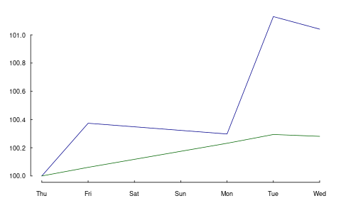
The argument when defines the origin.

  scale1(drax, when = 3, level = 100)

         dax    rexp
[1,]  99.703  99.769
[2,] 100.076  99.830
[3,] 100.000 100.000
[4,] 100.829 100.062
[5,] 100.741 100.049
attr(,"scale1_origin")
[1] 3

This origin is attached to the scaled series as an attribute scale1_origin. This is useful if you want mark the start of the scaled series; for instance, in a plot with abline.

With a zoo object, when should be compatible with the class of the object's index.

  scale1(drax.zoo, when = as.Date("2014-01-07"), level = 100)

               dax    rexp
2014-01-02  98.883  99.707
2014-01-03  99.253  99.768
2014-01-06  99.177  99.938
2014-01-07 100.000 100.000
2014-01-08  99.912  99.987
attr(,"scale1_origin")
[1] 2014-01-07

when also understands the keyword first.complete, which is actually the default, and the keywords first and last. first.complete is useful when some series have leading missing values.

drax[1:2, 1] <- NA
drax

        dax   rexp
[1,]     NA 440.53
[2,]     NA 440.79
[3,] 9428.0 441.55
[4,] 9506.2 441.82
[5,] 9497.8 441.76

scale1(drax, level = 100)   ## 'first.complete' is the default

        dax    rexp
[1,]     NA  99.769
[2,]     NA  99.830
[3,] 100.00 100.000
[4,] 100.83 100.062
[5,] 100.74 100.049
attr(,"scale1_origin")
[1] 3

When the argument centre is TRUE, the mean return is subtracted from the returns.

scale1(drax.zoo, centre = TRUE)

               dax    rexp
2014-01-02 1.00000 1.00000
2014-01-03 1.00114 0.99991
2014-01-06 0.99779 1.00091
2014-01-07 1.00348 1.00083
2014-01-08 1.00000 1.00000
attr(,"scale1_origin")
[1] 2014-01-02

The default is to subtract the geometric mean: the series will have a growth rate of zero; it will end where it started.

The argument scale takes a standard deviation and scales the returns to that standard deviation.

  apply(returns(scale1(drax.zoo, scale = 0.02)), 2, sd)

 dax rexp
0.02 0.02

This may create fairer comparisons, for instance, between fund prices that exhibit very different volatilities. It can also help to visualise correlation.

It should be stressed that centre and scale change returns, but scale1 expects and evaluates to levels (not returns).

The zoo method has a further argument that affects returns: inflate. To illustrate its use, let us create a constant series.

  z <- zoo(100,
           seq(from = as.Date("2015-1-1"),
               to   = as.Date("2016-1-1"),
               by   = "1 day"))
  head(z)
  tail(z)

2015-01-01 2015-01-02 2015-01-03 2015-01-04 2015-01-05 2015-01-06
       100        100        100        100        100        100

2015-12-27 2015-12-28 2015-12-29 2015-12-30 2015-12-31 2016-01-01
       100        100        100        100        100        100

inflate should be a numeric value: the annual growth rate that is added to the time-series's return (or that is subtracted from it, if negative).

head(scale1(z, inflate = 0.02))
tail(scale1(z, inflate = 0.02))

2015-01-01 2015-01-02 2015-01-03 2015-01-04 2015-01-05 2015-01-06
    1.0000     1.0001     1.0001     1.0002     1.0002     1.0003

2015-12-27 2015-12-28 2015-12-29 2015-12-30 2015-12-31 2016-01-01
    1.0197     1.0198     1.0198     1.0199     1.0199     1.0200

9.2. Scaling a series: how it works

The previous section provided examples of scaling series. In this section, we are going to see how scale1 does its computations.

First, a series $P$ passed to scale1 is transformed into returns, $R$. The scale argument allows you to set a desired volatility for the series's returns, defined as their standard deviation. The computation uses the fact that multiplying a random variable by a number $b$ changes its variance to $b^2$ times its original variance. Hence, scale1 divides the returns by the actual standard deviation and then multiplies them by the desired one (i.e. the value passed via the scale argument).

Changing total return (or, equivalently, average return) is slightly more complicated. Suppose we want to scale the total return of the series $P$ such that it equals some target return $r_*$. Start with writing the total return as the product of single-period returns.

\begin{equation} \label{eq:zret} \frac{P_1}{P_0}\frac{P_2}{P_1}\cdots\frac{P_T}{P_{T-1}}=\frac{P_T}{P_0} = (1+r_1)(1+r_2)(1+r_3)\cdots = \prod_{t=1}^T 1+r_t \end{equation}

There clearly is an infinity of possible adjustments that would do the trick. We might, for instance, change only $P_0$ or $P_T$ so that the desired return is achieved.

But that is probably not what we want. A reasonable requirement is that the scaling touches as few other statistical properties as possible. Adding a constant $z$ to the return in every period does that: it does not change the volatility of the returns; neither does it affect linear or rank correlation of the returns with some other series. To compute $z$, we need to solve the following equation:

\begin{equation} \label{eq:zret2} (1+r_1+z)(1+r_2+z)(1+r_3+z)\cdots = 1+r_* \end{equation}

Alternatively, we may use logs.

\begin{equation} \label{eq:zret3} \sum_i \log (1+r_i + z) = \log (1+r_*) \end{equation}

This is an application for root-finding (see chapter 11 of \citealp{Gilli2019}), for which scale1 uses uniroot.

10. Analysing trades

For some strategies or trading approaches, we may prefer to analyse trades, not equity series. (A case in point are intraday strategies, which have no exposure over night.) That is, we do not evaluate the strategy's performance at pre-defined, usually equally-spaced points in time, but rather split the trading history into separate trades.

10.1. Exposure

We have the following trades and times.

  amount <- c(1, 3, -3, 1, -3,  1)
  time   <- c(0, 1,  3, 4,  7, 12)

The holding period (duration) of these trades can be computed so:

  data.frame(position = cumsum(amount)[-length(amount)],
             from = time[-length(time)],
             to   = time[-1L],
             duration = diff(time))

  position from to duration
1        1    0  1        1
2        4    1  3        2
3        1    3  4        1
4        2    4  7        3
5       -1    7 12        5

We can plot the exposure.

  plot(c(time[1], time), cumsum(c(0, amount)),
       type = "s", xlab = "time", ylab = "position")

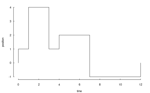
Thus, we have had a position from time 0 to time 12 (hours into the trading day, say), but its size varied. The function tw_exposure (time-weighted exposure) computes the average absolute exposure.

tw_exposure(amount, time)

1.75

To give a simpler example: suppose we bought at the open of a trading day and sold at noon. The average exposure for the day is thus half a contract.

amount <- c(1,  -1, 0)
time   <- c(0, 0.5, 1)
tw_exposure(amount, time)

0.5

If we bought at the open, went short at noon, and closed the position at the end of the day, the average exposure would be one contract, since absolute position size is relevant.

amount <- c(1, -2 , 1)
time   <- c(0,0.5,1)
tw_exposure(amount, time)

Whether absolute exposure is used is controlled by an argument abs.value. Setting it to FALSE can be useful to detect long or short biases.

tw_exposure(amount, time, abs.value = FALSE)

10.2. Splitting and rescaling

We have the following trades.

  timestamp <- 1:3
  amount <- c(-1, 2, -1)
  price <- c(100, 99, 101)

Calling split_trades will return a list of two single trades. Each single trade, in turn, is a list with components amount, price and timestamp.

  split_trades(amount = amount,
               price = price,
               timestamp = timestamp,
               aggregate = FALSE)

[[1]]
[[1]]$amount
[1] -1  1

[[1]]$price
[1] 100  99

[[1]]$timestamp
[1] 1 2


[[2]]
[[2]]$amount
[1]  1 -1

[[2]]$price
[1]  99 101

[[2]]$timestamp
[1] 2 3

Note that the second transaction (buy 2 @ 99) has been split up: buying one contract closes the first trade; the other contract opens the second trade. This splitting is useful in its own right: there are accounting systems around that cannot handle a trade that switches a position directly from long to short, or vice versa. Instead, the trade needs first be closed (i.e. the net position becomes zero).

With argument aggregate set to TRUE, the function reconstructs the total series, but with those trades splitted that change the position's sign.

split_trades(amount, price, timestamp, aggregate = TRUE)

$amount
[1] -1  1  1 -1

$price
[1] 100  99  99 101

$timestamp
[1] 1 2 2 3

Another example. We have the following trades and impose a limit that the maximum absolute exposure for the trader should only be 2.

timestamp <- 1:6
amount <- c(-1,-1,-1,1,1,1)
price <- c(100,99,98,98,99,100)
limit(amount, price, timestamp, lim = 2)

$amount
[1] -1 -1  1  1

$price
[1] 100  99  99 100

$timestamp
[1] 1 2 5 6

Scaling the trades.

scale_to_unity(amount)

[1] -0.333 -0.333 -0.333  0.333  0.333  0.333

Closing the trade at once.

close_on_first(amount)

[1] -1 -1 -1  3  0  0

11. Plotting irregularly-spaced series during trading hours

11.1. An example

We have the following sample of prices of the Bund future contract, traded at the Eurex in Germany.

times	prices
2012-10-18 20:00:09	139.82
2012-10-18 20:01:11	139.82
2012-10-18 20:01:59	139.8
2012-10-18 20:01:29	139.81
2012-10-18 20:16:49	139.77
2012-10-18 20:50:49	139.85
2012-10-18 21:23:19	139.76
2012-10-18 21:41:39	139.76
2012-10-18 21:59:59	139.77
2012-10-19 09:16:10	139.8
2012-10-19 09:49:31	139.86
2012-10-19 21:12:49	140.46
2012-10-19 21:42:31	140.39
2012-10-22 08:45:15	140.14
2012-10-22 09:05:33	140.15

(You'll find the code to generate those times in the code file for this chapter.)

Note that I have left the time zone to the operating system. Since my computer is typically located in the time zone that the tz database (https://www.iana.org/time-zones)

calls 'Europe/Zurich', the first time should be 2012-10-18 20:00:09. If, for instance, your computer is in 'America/Chicago' instead and you run the above code, the first time would be 2012-10-18 13:00:09. Which is right: it is the correct time, only translated into Chicago local time.

A plot of price against time looks like this.

  plot(times, prices, type = "s")

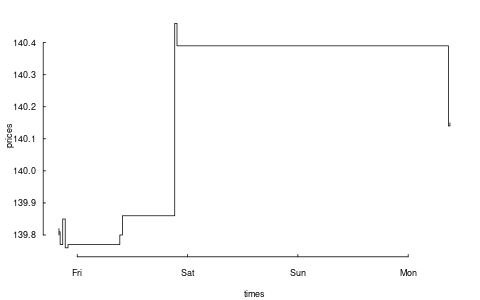
Such a plot is fine for many purposes. But the contract for which we have prices is only traded from Monday to Friday, not on weekends, and it is traded only from 08:00 to 22:00 Europe/Berlin time. So the plot should omit those times at which no trading takes place. This is what the function plot_trading_hours does.

  tmp <- plot_trading_hours(x = prices, t = times,
                            interval = "1 sec",
                            labels = "day",
                            fromHHMMSS = "080000",
                            toHHMMSS = "220000",
                            type = "s")

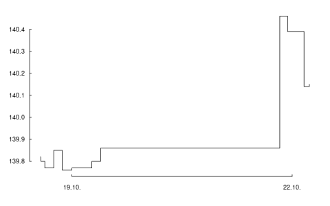
What we need for such a plot is a function that maps actual time to a point on the x-scale, while the y-scale stays unchanged. If we were talking only about days, not times, we needed something like this:

day	x-position	mapped x-position
Thursday	1	1
Friday	2	2
Saturday	3	`<removed>`
Sunday	4	`<removed>`
Monday	5	3

This mapping is what plot_trading_hours provides. And not much more: the design goal of the function is to make it as much as possible an ordinary plot; or more specifically, to make it as similar as possible to the plot function. Indeed, plot_trading_hours calls plot with a small number of default settings:

list(type = "l", xaxt = "n", xlab = "", ylab = "")

These settings can all be overridden through the ... argument, which is passed to plot. Note that we already set s as the plot's type in the last code chunk. The only required setting is suppressing the x-axis with setting xaxt to 'n', because plot_trading_hours will create its own x-axis via a call to axis(1, ...). In case you wish to use your own axis specification, either set do.plotAxis to FALSE or pass settings to axis through the list axis1.par.

11.2. More examples

11.2.1. Value of `plot_trading_hours`

Like plot, plot_trading_hours is typically called for its side effect: creating a plot. But it also returns useful information (invisibly, unless called with do.plot = FALSE).

str(tmp)

List of 6
 $ t          : int [1:15] 1 63 81 111 1001 3041 4991 6091 7191 ...
 $ x          : num [1:15] 140 140 140 140 140 ...
 $ axis.pos   : num [1:2] 7193 57594
 $ axis.labels: chr [1:2] "19.10." "22.10."
 $ timegrid   : POSIXct[1:61527], format: "2012-10-18 20:00:09" ...
 $ map        : function (t)

This information can be used to add elements to plots. An example follows.

11.2.2. Adding grid lines

We can add grid lines with abline. The y-axis poses no special problem. The positions of the x-axis ticks are returned from plot_trading_hours.

  tmp <- plot_trading_hours(x = prices, t = times,
                          interval = "1 sec",
                          labels = "day",
                          fromHHMMSS="080000",
                          toHHMMSS = "220000",
                          type = "s")
  abline(h = axTicks(2), v = tmp$axis.pos,
         col = "lightgrey", lty = "dotted")

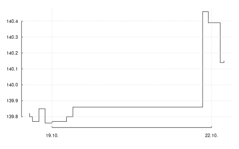
If we want to mark a specific time, say 19 October, 13:10:23, we can use the function map that the call to plot_trading_hours returns. We first create the specific time with, for example, ISOdatetime or strptime.

  ## Again, I do not specify a time zone since time zones
  ## depend on the operating system. To reproduce the
  ## example, you may use this representation:
  ##
  ## mytime <- structure(1350645023,
  ##                     class = c("POSIXct", "POSIXt"),
  ##                     tzone = "")

  mytime <- ISOdatetime(2012, 10, 19, 13, 10, 23)
  mytime

[1] "2012-10-19 13:10:23 CEST"

Now we use map to translate this time into the appropriate x-position.

  tmp <- plot_trading_hours(x = prices, t = times,
                          interval = "1 sec", labels = "day",
                          fromHHMMSS="080000",
                          toHHMMSS = "220000",
                          type = "s")
  abline(h = axTicks(2), v = tmp$axis.pos,
         col = "lightgrey", lty = "dotted")
  abline(v = tmp$map(mytime)$t, col = "red")

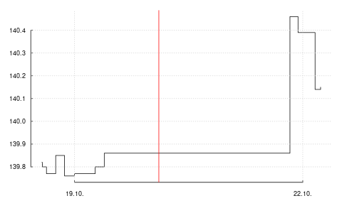
The function map returns a list with two components, t and ix.

tmp$map(mytime)

$t
[1] 25816

$ix
[1] 1

The first component is the appropriate position on the x-axis; since it is a time it is called t. The second component gives the subscripts to values that should actually be plotted. As an example, suppose that we wish to plot points at several prices at 21:00:00 for several days.

  ## moretimes <- structure(c(1350586800, 1350673200, 1350759600),
  ##                        class = c("POSIXct", "POSIXt"), tzone = "")
  ##

  moretimes <- ISOdatetime(2012, 10, 18:20, 21, 00, 00)
  values <- seq(140, 140.20, length.out = length(moretimes))
  data.frame(times = moretimes,
             weekday = format(moretimes, "%A"),
             values)

                times  weekday values
1 2012-10-18 21:00:00 Thursday  140.0
2 2012-10-19 21:00:00   Friday  140.1
3 2012-10-20 21:00:00 Saturday  140.2

But 20 October 2012 is a Saturday, and so it does not appear in the plot.

  tmp$map(moretimes)

$t
[1]  3592 53993

$ix
[1] 1 2

The values that should be plotted can conveniently be found by using ix.

values[tmp$map(moretimes)$ix]

[1] 140.0 140.1

11.3. Daily data

plot_trading_hours also handles data on a daily frequency. The function will assume such a case if the timestamp is of class Date; it will then choose sensible defaults for the time-axis. In effect, the function will remove weekends and, if specified, holidays.

As an example, consider the first 10 observations of the DAX dataset.

  x <- DAX[1:10, ]
  t <- as.Date(row.names(DAX)[1:10])
  data.frame(t, x, weekday = weekdays(t))

If we plot these data, there will be a value plotted for 2014-01-04, as marked by the vertical line.

  plot(t, x, type = "l")
  abline(v = as.Date("2014-01-04"))

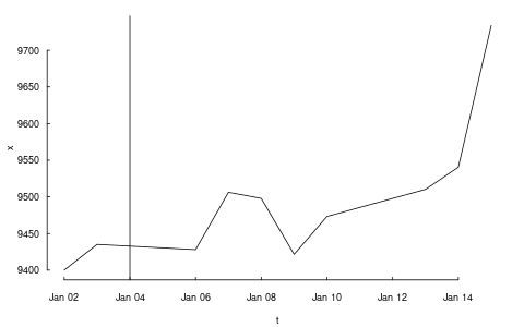
That is despite the fact that this is a Saturday.

   format(as.Date("2014-01-04"), "%A")

Saturday

This is not a bug: it is the default behaviour of plot. Saturday's value results from an interpolation. plot_trading_hours instead ignores such nonexisting dates.

   plot_trading_hours(x, t)

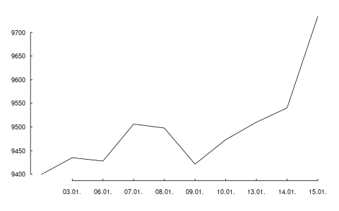
12. Valuation

Computing the value of a position is, in principle, straightforward: multiply the prices of assets by the numbers of contracts you hold and sum the resulting values.

This immediately leads to three questions:

What is the price?
What is a contract?
Are we allowed to sum?

12.1. Prices

Valuing an instrument can mean using either a market price or a theoretical price. In the discussion that follows, I will assume that we already have prices (or net-present values).

13. Other Tools

13.1. Dividend adjustments

The function div_adjust corrects price series for dividends. It is meant as a low-level function and is implemented to work on numeric vectors. Consider a hypothetical price series x, which goes ex-dividend at time 3.

  x <- c(9.777, 10.04, 9.207, 9.406)
  div <- 0.7
  t <- 3

The default for div_adjust is to match the final price.

  div_adjust(x, t, div)

[1] 9.086185 9.330603 9.207000 9.406000

If you prefer a correction that matches the first price, set argument backward to FALSE.

  div_adjust(x, t, div, backward = FALSE)

[1]  9.77700 10.04000  9.90700 10.12113

13.2. Stocks splits

The function split_adjust handles stock splits. It is implemented to work on numeric vectors.

13.3. Treasuries quotes

US treasury bonds are often quoted in 1/32nds of points. For instance, the price 110'030 would mean 110+3/32.

The function quote32 lets you parse and `pretty-print' such prices.

quote32(c("110-235", "110-237"))

[1] 110-23+ 110-23¾

Internally, quote32 will store the prices as numeric values: the fractions are only used for printing.

as.numeric(quote32(c("110-235", "110-237")))

[1] 110.73 110.74

dput(quote32(c("110-235", "110-237")))

structure(c(110.734375, 110.7421875),
          handle = c(110, 110),
          ticks = c(23, 23),
          fraction = c(2, 3),
          class = "quote32")

13.4. Validating security identification numbers

An ISIN, which stands for International Securities Identification Number, uniquely¹⁵ identifies a security.

  is_valid_ISIN(c("DE0007236101",     ## Siemens
                  "DE0007236102"))    ## last digit changed

[1]  TRUE FALSE

There is a function is\_valid\_SEDOL too.

13.5. Price tables

A pricetable is a matrix of prices, with some added functionality for subsetting.

13.6. Trees

To normal people, a tree consists of a trunc, branches and leaves. To people who do graph theory, a tree is a connected graph with only one path between any two nodes.

Trees are useful to represent hierachies – just think of a file tree. For portfolios, a tree can be used to indicate groupings, such as countries or industries. (See argument account in function position.)

14. FAQ/FRC (Frequently-required computations)

I have a list of timestamped trades and I need to compute P/L between two points in time, for instance between yesterday's evening close and now (intraday).

Call the points in time $t_0$ and $t_1$. The easiest case is if there were no positions at both $t_0$ and $t_1$. In that case, create a journal of your trades, and call pl.

If there were positions, you will need the valuation prices for all instruments with positions at both points in time. Then, you can use pl; see arguments initial.position and vprice.

Alternatively, you would arrive at the P/L as follows:

Compute the position at $t_0$ and make it a journal $J_0$. The prices need to be the valuation prices. (That is, pretent you opened the position at their valuation prices at $t_0$.)
Take all transactions at $t > t_0$ and $t \leq t_1$ and put them into a journal $J$.
Compute the position at $t_1$ make it a journal $J_1$, and multiply all amounts by -1. The prices need to be the valuation prices. (That is, pretent you closed the position at their valuation prices at $t_1$.)
Combine $J_0$, $J$, and $J_1$ and compute the P/L.

How can I compute portfolio returns when I don't have prices, but only returns of the assets?

Compute artificial prices; e.g. using something like

P <- cumprod(c(1, 1 + R))

Then feed those series to returns.

I have a portfolio with constant weights. How to compute its returns when it is rebalanced at specific times?

Compute artificial prices, and then use returns: see arguments weights and rebalance.when. See Section Portfolio returns.

I have a journal of trades and want to compute the number of trades per day?

Use tapply. If the timestamp inherits from class Date or can be coerced to Date, the following line will compute the number of trades per day.

tapply(J, as.Date(J$timestamp), length)

Backtesting: How do I access the current weights of the portfolio?

btest is based on prices. You can compute returns easily within signal:

  Close()*Portfolio()/Wealth()

I have a list of trades: instrument, side (buy/sell), quantity, when and at what price. How to compute the profit and loss for each?

See pl.

I have a list of trades in an instrument and want to plot these trades against the price of the traded instrument.

Use pl; in particular, pass the prices with vprice.

I have a signal series (+1, 0, 0, +1, …), and need to transform it into a profit-and-loss series.

If these are positions, pass the signals to btest and access them with signals[Time()].

I need to determine the month-to-date profit-and-loss.

compute position on last day of last month
make journal from position (add prices)
combine with journal since month start
use ~pl on all instruments

btest: I want to print my current P/L in every period.

Use print.info.

btest: I invest in assets that pay accrued interest.

Directly work with the dirty prices. If the signals depend on clean prices, pass them as extra information and access them with clean_price[Time()]. Alternatively, work with the clean prices, and use cashflow to add the accrued interest to the cash account.

btest: Can I rebalance more frequently than I compute a signal?

You can, but it does not make sense in the standard setup. That is, no rebalancing will take place, even if you instruct btest to do so. The reason is that a signal computes a suggested position (in units of the instrument); once this position has been built up, no more trading is required. This is even true when using weights: The argument convert.weights is a convenience that converts weights into a suggested position; btest does not store these weights, only the suggested position.

15. Appendix: Classes and data structures

The following classes are implicitly defined (i.e. they are S3 classes):

journal: keeps transactions. Internally, a object of class journal is named list of atomic vectors.
position: the numerical positions of different accounts/instruments at specific points in time. Always stored in a numeric matrix with attributes timestamp and instrument; points in time are in rows, instruments in columns.
period returns: numeric vector (potentially a matrix) with attributes timestamp and period. The class is called p_returns
instrument: term sheet (description etc); it does know nothing about market data – not yet implemented
cashflow: internal – not yet implemented
NAVseries: store a time-series of net asset values
pricetable: a matrix of NAVs (or prices); each column corresponds to one asset. Additional attributes instrument and timestamp. Often, pricetables will be created corresponding to positions.

16. Appendix: Notes for developers

16.1. Methods for `returns`

Methods are responsible for 'stripping' the input down do x and t, calling 'returns.default' or some other method, and then to re-assemble the original class's structure. When period is not specified, methods should keep timestamp information for themselves and not pass it on. That is, returns.default should only ever receive a timestamp when period is specified.

17. Appendix: Date and time in R

17.1. Dates in R

Vectors of class Date give the number of days that have passed since 1 January 1970, with dates before that date represented by negative numbers.

unclass(as.Date("1970-1-1"))

[1] 0

unclass(as.Date("1969-1-1"))

[1] -365

While Dates are conceptually integers, their representation does not ensure that they really are: fractions of a day are ignored for printing, but they are not removed. That can give rise to subtle errors. Suppose, for instance, you wanted to select a date that is a little more than one year before another date. You could to this as follows.

   x0 <- as.Date("2016-11-01") - 365*1.05
   x0

[1] "2015-10-14"

But the printed date is not going to match a Date created from character.

   match(as.Date("2015-09-14"), x0)

[1] NA

That is because x0 will (silently) keep its fractional part.

dput(as.Date("2015-09-26"))
dput(x0)

structure(16704, class = "Date")
structure(16722.75, class = "Date")

So, whenever you plan to match or compare Dates, make sure that they are integers.

   match(as.Date("2015-10-14"), trunc(as.Date("2016-11-01") - 365*1.05))

[1] 1

Or coerce to character, which is often safer.

   match(as.character("2015-10-14"),
         as.character(as.Date("2016-11-01") - 365*1.05))

[1] 1

17.2. From a vector of Dates, extract the last day of each month

   d <- seq(as.Date("2010-1-1"),
            as.Date("2012-12-15"),
            by = "1 week")

If the Dates are sorted, use aggregate with tail. (If the Dates come from a zoo object, they will always be sorted.)

   aggregate(d,
             by = list(format(d, "%Y-%m")),
             FUN = tail, 1L)[[2L]]

[1] "2010-01-29" "2010-02-26" "2010-03-26" "2010-04-30"
[5] "2010-05-28" "2010-06-25" "2010-07-30" "2010-08-27"
[9] "2010-09-24" "2010-10-29"
[ reached getOption("max.print") -- omitted 26 entries ]

If the Dates are not sorted, either sort them

   if (is.unsorted(d))
       d <- sort(d)

or use max.

   d <- sample(d, size = length(d))
   aggregate(d, by = list(format(d, "%Y-%m")), FUN = max)[[2L]]

[1] "2010-01-29" "2010-02-26" "2010-03-26" "2010-04-30"
[5] "2010-05-28" "2010-06-25" "2010-07-30" "2010-08-27"
[9] "2010-09-24" "2010-10-29"
[ reached getOption("max.print") -- omitted 26 entries ]

The code also works when dates are duplicated.

17.3. From a vector of Dates, extract the first day of each month

As before, but sort in descending order or use min.

17.4. Compute the week number and start/end of week

From R-help.

   iso_start_end <- function(d) {
       d <- as.Date(d)
       wday <- as.POSIXlt(d)$wday
       wday[wday == 0] <- 7
       data.frame(date = d,
                  week = format(d, "%V"),
                  starts = d - wday + 1,
                  ends = d + 7 - wday)
   }

   d <- c("2010-08-21", "2010-08-22",
          "2010-08-23", "2010-08-24")
   iso_start_end(d)

        date week     starts       ends
1 2010-08-21   33 2010-08-16 2010-08-22
2 2010-08-22   33 2010-08-16 2010-08-22
3 2010-08-23   34 2010-08-23 2010-08-29
4 2010-08-24   34 2010-08-23 2010-08-29

17.5. Dates in JavaScript

console.log(Date(2016, 0, 18, 10, 11, 12));

Fri Jan 20 2017 10:48:26 GMT+0100 (CET)

17.6. Time

Unix time, the number of seconds since 1970-01-01 00:00:00 UTC. Traditionally, represented as a 4-byte integer.

17.7. Unix timestamps in the Bourne shell

date        ## current time
date +%s

Tue 12 Mar 14:56:56 CET 2024
1710251816

Convert back to human-readable time.

date --date='@1710251816'

Tue 12 Mar 14:56:56 CET 2024

17.8. Unix timestamps in R

R represents the timestamp as doubles.

   (tmp <- unclass(Sys.time()))

1473428055.30705

Convert back to human-readable time.

   .POSIXct(tmp)

2016-09-09 15:34:15

18. Appendix: R and package versions used

R version 4.2.2 Patched (2022-11-10 r83330)
Platform: x86_64-pc-linux-gnu (64-bit)
Running under: Ubuntu 22.10

Matrix products: default
BLAS:   /usr/lib/x86_64-linux-gnu/openblas-openmp/libblas.so.3
LAPACK: /usr/lib/x86_64-linux-gnu/openblas-openmp/libopenblasp-r0.3.20.so

locale:
 [1] LC_CTYPE=en_US.UTF-8       LC_NUMERIC=C
 [3] LC_TIME=en_GB.UTF-8        LC_COLLATE=en_US.UTF-8
 [5] LC_MONETARY=en_GB.UTF-8    LC_MESSAGES=en_US.UTF-8
 [7] LC_PAPER=en_GB.UTF-8       LC_NAME=C
 [9] LC_ADDRESS=C               LC_TELEPHONE=C
[11] LC_MEASUREMENT=en_GB.UTF-8 LC_IDENTIFICATION=C

attached base packages:
[1] stats     graphics  grDevices utils     datasets  methods
[7] base

other attached packages:
[1] rbenchmark_1.0.0 orgutils_0.5-0   NMOF_2.8-0
[4] zoo_1.8-11       PMwR_0.19-0

loaded via a namespace (and not attached):
[1] datetimeutils_0.6-0 compiler_4.2.2      tools_4.2.2
[4] parallel_4.2.2      fastmatch_1.1-3     grid_4.2.2
[7] textutils_0.3-1     lattice_0.20-45

Footnotes:

The package was called PM until 2012. Also, much of its functionality has over the years been moved to separate packages, of which several made their way to CRAN, such as datetimeutils, mailtools, textutils and tsdb.

A great inspiration for `smallness' were the principles behind the tools that make working on a Unix-type operating system so productive (and so much fun). In particular, that a programme should do one thing only (but thoroughly). Another inspiration came from the Lua language, which I used much in the past. Lua even removed functions to make the language even smaller. Closer to finance, there is the Ledger project.

Only similar: a data-frame may contain non-atomic vectors, a.k.a. lists.

⁴

Numbers have to be converted to character in some situations, for instance when used as names.

⁵

This notation is inspired by the syntax of ledger files. See https://www.ledger-cli.org/ .

⁶

The behaviour of `[[` may change in the future: it may then be used to iterate over the transactions in a journal, not the fields. This would be motivated by https://developer.r-project.org/blosxom.cgi/R-devel/NEWS/2016/03/09 even though the commit was reversed two days later https://developer.r-project.org/blosxom.cgi/R-devel/NEWS/2016/03/11

⁷

In an earlier version of the code, average buy/sell price did not take into account vprice. But specifying vprice creates a fiction, anyway (P/L 'as if' the trade was closed), and this fiction is more informative if the average buy/sell price is adjusted.

⁸

The function never computes logarithmic returns. See A digression on logarithmic returns.

⁹

See Vectorization.

¹⁰

In case you did not know: drax is not only the name of a dataset in this book, but also the name of Marvel-comics superhero and of the villain of a James Bond novel. The latter is actually German, which makes it obvious to choose the name for representing German indices. :-)

¹¹

Unqualified statements such as `R is slow' or `loops are slow' are not useful. In the current version of PMwR, the overhead of running a backtest with btest with 500 assets and 5000 observations (and rebalancing each of those assets at each of those 5000 timestamps) is less than five seconds; if only few assets are touched, overhead is less than one second.

¹²

Remember what Brian Kernighan said: Everyone knows that debugging is twice as hard as writing a program in the first place. So if you're as clever as you can be when you write it, how will you ever debug it?

¹³

An example of a statistic that cannot be computed in a robust way is a beta coefficient – or, in fact, any other multivariate statistic. Such numbers will depend on a chosen benchmark, and what is more, they typically need careful checking because of asynchronous time-series: A mutual fund's NAV that is published with a delay may show little correlation with a stock-market index (when matched on time-stamps), but that is only because of the 'attenuation bias', which skews the correlation towards zero.

¹⁴

Transformating or scaling data are a key element of exploratory data analysis in general. See Tukey's EDA (1977). TODO: find H. Simon reference on scaling (taking reciprocal value). See also \citet{schumann2013b}.

¹⁵

More or less uniquely, depending on the definition of security. ISINs are widely used for equities, in particular in European markets. But note that ISINs do not contain information about the trading venue. Also, for derivatives, an ISIN may not uniquely identify the contract: for instance, Euro-Bund Futures, traded at the Eurex, have a single ISIN for all maturities.

1. Introduction

1.1. About PMwR

1.2. Principles

1.3. Setting up R

1.4. Typographical conventions

2. Keeping track of transactions: journals

2.1. Overview

2.2. Fields

2.3. Creating and combining journals

2.4. Selecting transactions

2.5. Computing balances

2.5.1. Computing positions from journals

2.5.2. Algorithms for computing balances

2.5.2.1. when and timestamp sorted

2.5.2.2. when and timestamp unsorted

2.6. Aggregating and transforming journals

3. Computing profit and loss

3.1. Simple cases

3.1.1. Total profit/loss

3.1.2. P/L over time

3.2. More-complicated cases

4. Computing returns

4.1. Simple returns

4.2. A digression on logarithmic returns

4.3. Holding-period returns

4.4. Portfolio returns

4.5. Return contribution

4.6. Returns when there are external cashflows

5. Backtesting

5.1. Decisions

5.2. Data structure

5.3. Function arguments

5.3.1. Available information within functions

5.3.2. Function arguments

5.4. Examples: A single asset

5.4.1. A useless first example

5.4.2. More-useful examples

5.4.2.1. Passing environments

5.5. Examples: Several assets

5.5.1. A simple example

5.6. Miscellaneous

5.6.1. Handling missing values

5.6.2. Distributing backtest computations

5.6.3. Remembering an entry price

5.6.4. Delaying signals

5.6.5. Specifying when to compute a signal and trade

5.6.6. Writing a log

5.6.7. Selecting parameters: calling btest recursively

5.6.8. Time-varying asset universes

6. Backtesting strategies in parallel

6.1. Distributed computing

6.2. Loops and apply functions

6.3. Distributing data

6.4. Distributing data, continued

7. Rebalancing a portfolio

7.1. Usage with unnamed vectors

7.2. Usage with named vectors

7.3. Usage with positions

7.4. Constructive methods: An example

7.5. Algorithms

7.6. Substituting a basket by its components

8. Summarising portfolio time-series

8.1. Creating NAV series

8.2. Summarising NAV series

8.3. More than one series

8.4. Drawdowns and Streaks

8.4.1. Drawdown

8.4.2. Streaks

9. Scaling series

9.1. Examples

9.2. Scaling a series: how it works

10. Analysing trades

10.1. Exposure

10.2. Splitting and rescaling

11. Plotting irregularly-spaced series during trading hours

11.1. An example

11.2. More examples

11.2.1. Value of plot_trading_hours

11.2.2. Adding grid lines

11.3. Daily data

5.6.7. Selecting parameters: calling `btest` recursively

6.2. Loops and `apply` functions

11.2.1. Value of `plot_trading_hours`

16.1. Methods for `returns`