Restarting Nelder-Mead

We describe a simple method to improve the results of Nelder–Mead direct search: instead of relying on a single run with possibly many iterations, we restart the search (ie, re-initialise the simplex) several times. While it is impossible to give advice like 'this is always better than that', the restart-strategy is easy to test; thus, for a given problem we can run little experiments to find out whether it should be used. Here is one such experiment.

We load and attach the NMOF package.

require("NMOF")      ## attach the package

An example problem, the Rosenbrock function. The minimum is at x==1; the minimum function value is zero.

OF <- tfRosenbrock   ## see ?testFunctions
size <- 20L          ## the problem size
x <- rep(1, size)    ## the (known) solution
OF(x)                ## ... and associated OF value

[1] 0

How many steps would Nelder-Mead need to signal convergence? (Note that we do not require actual convergence; we just want to know after how many iterations the algorithm stops.) To find out, we run a little experiment.

iterStop <- numeric(1000L)
for (i in seq(along.with = iterStop)) {
    x0 <- rnorm(size)
    sol <- optim(x0, OF, control = list(maxit = 1e6))
    iterStop[i] <- sol$counts[1L]
}
summary(iterStop)

   Min. 1st Qu.  Median    Mean 3rd Qu.    Max.
   3671    7638    9332    9782   11410   27500

The summary command should give a result like this (it will differ because of the random starting values).

Now we try to minimise the Rosenbrock function. We test two strategies: strategy 1 uses a single restart with at most 25.000 function evaluations from a random initial solution. strategy 2 uses the same initial solution, but 4 additional restarts, each starting from the last returned solution. We set up strategy 2 such that it will, at most, use the same number of function evaluations as strategy 1.

trials <- 1000L
res1 <- numeric(trials) ## results of strategy 1
res2 <- numeric(trials) ## results of strategy 2

for (i in seq_len(trials)) {

    ## random initial solution: same for type 1 and type 2
    x0 <- rnorm(size)

    ## strategy 1 -- single run
    sol <- optim(x0, OF, control = list(maxit = 25000))
    feval <- sol$count[1L] ## iterations needed
    res1[i] <- sol$value

    ## strategy 2 -- restart
    for (j in 1:5) {
        sol <- optim(x0, OF, control = list(maxit = trunc(feval/5)))
        x0 <- sol$par
    }
    res2[i]<- sol$value
}

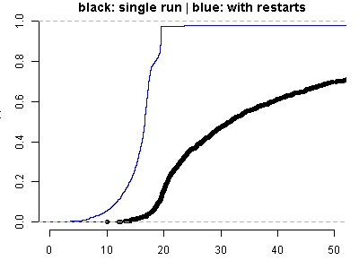
Finally, we plot the results.

par(mar = c(3,3,1,1), bty = "n")
plot(ecdf(res1), xlim = c(0,50), ylim = c(0,1),
     main = "black: single run | blue: with restarts")
lines(ecdf(res2), col = "blue")

return to main page...

---