Path-dependent strategies

In this note I show how a simple path-dependent strategy – a stop loss – can be implemented with btest. To keep it simple, we look only at the univariate case, i.e. a single time-series. For data, we use the time-series of the DAX (a German stock-market index), which is included in the PMwR package.

library("PMwR")

prices <- c(DAX[[1]])
timestamp <- as.Date(row.names(DAX))

The first strategy: buy once, on the first timestamp, and then sell if the price moves more than stop.loss percent below the entry price.

buy_once_SL <- function(stop.loss) {
    if (Time(0) == 1) {        
        Globals$entry <- Close(0)
        1
    } else if (Portfolio() && Close() < Globals$entry * (1 - stop.loss))
        0
}

bt.buy_once_SL <- btest(prices = prices,
                        signal = buy_once_SL,
                        timestamp = timestamp,
                        stop.loss = 0.05,
                        b = 0)

journal(bt.buy_once_SL)

   instrument   timestamp  amount    price
1     asset 1  2014-01-02       1  9400.04
2     asset 1  2014-10-13      -1  8812.43

2 transactions

Remarks: Since we have a calendar schedule when to buy, there is no need for a burnin, so b is set to zero. Also, within the signal function, we test whether Time(0) equals 1, i.e. we use no lag. The else clause starts with the test Portfolio(): If we are not invested (i.e. we have been stopped out), the position will be zero, which evaluates to FALSE. For this example, such a test would not have been necessary, since the second condition is very fast to compute. But in general, for a path-dependent strategy, btest needs to loop through every single data point, and then not doing unnecessary work helps to speed up things.

Suppose we had wanted a trailing stop, i.e. sell when stop.loss percent below the highest price observed after the position was opened. In that case, we simply would have to update the entry price (which should then better be named high or reference or something similar). This update would have to happen whenever we have an open position. In any case, the entry is stored in Globals, which is an environment provided by btest. For our purposes, we can treat it just like a list, only that it is never copied. Thus, the objects we put into it are not local, but are persistent between invocations of the signal function.

In the example above, once we have closed the position, we will never again invest. Suppose that instead, we would want to reinstate a new position at the first day of every quarter. We would need only few changes to buy_once_SL.

library("datetimeutils")
trade.dates <- nth_day(timestamp, period = "quarter", n = "first")

buy_quarterly_SL <- function(stop.loss, trade.dates) {
    if (Timestamp(0) %in% trade.dates) {
        Globals$entry <- Close(0)
        1
    } else if (Portfolio() && Close() < Globals$entry * (1 - stop.loss))
        0
}

bt.buy_quarterly_SL <- btest(prices = prices,
                             signal = buy_quarterly_SL,
                             timestamp = timestamp,
                             stop.loss = 0.05,
                             trade.dates = trade.dates,
                             b = 0)

journal(bt.buy_quarterly_SL)

   instrument   timestamp  amount     price
1     asset 1  2014-01-02       1   9400.04
2     asset 1  2014-08-04      -1   9154.14
3     asset 1  2014-10-01       1   9382.03
4     asset 1  2014-10-13      -1   8812.43
5     asset 1  2015-01-02       1   9764.73
6     asset 1  2015-05-06      -1  11350.15
7     asset 1  2015-07-01       1  11180.50
8     asset 1  2015-08-21      -1  10124.52
9     asset 1  2015-10-01       1   9509.25

9 transactions

Note that with this specification, the entry price is updated every quarter, even when we have not been stopped out.

Finally, we may want to compare the results with a buy-and-hold strategy. The signal function is so simple that we can inline it.

bt.buy_hold <- btest(prices = prices,
                     signal = function() 1,
                     timestamp = timestamp,
                     b = 0)

journal(bt.buy_hold)

   instrument   timestamp  amount    price
1     asset 1  2014-01-02       1  9400.04

1 transaction

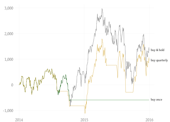
We plot the resulting equity curves.

library("plotseries")  ## https://github.com/enricoschumann/plotseries
library("zoo")
plotseries(merge(as.zoo(NAVseries(bt.buy_hold)),
                 as.zoo(NAVseries(bt.buy_once_SL)),
                 as.zoo(NAVseries(bt.buy_quarterly_SL))),
           add0 = TRUE,
           add1 = FALSE,
           col = c(grey(0.5), "darkgreen", "goldenrod3"),
           labels = c("buy & hold", "buy once", "buy quarterly"),
           add.returns = FALSE,
           add.dollars = FALSE,
           big.mark = ",")